Simple linear regression Archives

Simple linear regression is the most basic form of regression. It is the foundation of statistical or machine learning modelling technique. All advance techniques you may use in future will be based on the idea and concepts of linear regression. It is the most primary skill to explore your data and have the first look into it.

Simple linear regression is a statistical model which studies the relationship between two variables. These two variables will be such that one of them is dependent on the other. A simple example of such two variables can be the height and weight of the human body. From our experience, we know that the bodyweight of any person is correlated with his height.

The body weight changes as the height changes. So here body weight and height are dependent and independent variable respectively. The task of simple linear regression is to quantify the change happens in the dependent variables for a unit change in the independent variable.

Mathematical expression

We can express this relationship using a mathematical equation. If we express a person’s height and weight with X and Y respectively, then a simple linear regression equation will be:

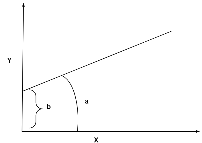
Y=a.X+b

With this equation, we can estimate the dependent variable corresponding to any known independent variable. Simple linear regression helps us to estimate the coefficients of this equation. As a is known now, we can say for one unit change in X, there will be exactly a unit change in Y.

See the figure below, the a in the equation is actually the slope of the line and b is the intercept from X-axis.

As the primary focus of this post is to implement simple linear regression through Python, so I would not go deeper into the theoretical part of it. Rather we will jump straight into the application of it.

Before we start coding with Python, we should know about the essential libraries we will need to implement this. The three basic libraries are NumPy, pandas and matplotlib. I will discuss about these libraries briefly in a bit.

Application of Python for simple linear regression

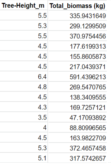
I know you were waiting for this part only. So, here is the main part of this post i.e. how we can implement simple linear regression using Python. For demonstration purpose I have selected an imaginary database which contains data on tree total biomass above the ground and several other tree physical parameters like tree commercial bole height, diameter, height, first forking height, diameter at breast height, basal area. Tree biomass is the dependent variable here which depends on all other independent variables.

Here is a glimpse of the database:

From this complete dataset, we will use only Tree_height_m and Tree_biomass (kg) for this present demonstration. So, here the dataset name is tree_height and has the look as below:

Python code for simple linear regression

Importing required libraries

Before you start the coding, the first task is to import the required libraries. Give them a short name to refer them easily in the later part of coding.

import pandas as pd
import numpy as np
import matplotlib.pyplot as plt

These are the topmost important libraries for data science applications. These libraries contain several classes and functions which make performing data analysis tasks in Python super easy.

For example, numPy and Pandas are the two libraries which encapsulate all the matrix and vector operation functions. They allow users to perform complex matrix operations required for machine learning and artificial intelligence research with a very intuitive manner. Actually the name numPy comes from “Numeric Python”.

Whereas Matplotlib is a full-fledged plotting library and works as an extension of numPy. The main function of this library to provide an object-oriented API for useful graphs and plots embedded in the applications itself.

These libraries get automatically installed if you are installing Python from Anaconda, which is a free and opensource resource for R and Python for data science computation. So as the libraries are already installed you have to just import them.

Importing dataset

dataset=pd.read_csv('tree_height.csv')
x=dataset.iloc[:,:-1].values
y=dataset.iloc[:, 1].values

Before you use this piece of code, make sure the .csv file you are about to import is located in the same working directory where the Python file is located. Otherwise, the compiler will not be able to find the file.

Then we have to create two variables to store the independent and dependent data. Here the use of matrix needs special mention. Please keep in mind that the dataset I have used has the dependent (Y) variable in the last column. So, while storing the independent variable in x, the last column is excluded and for dependent variable y, the location of the last column is considered.

Splitting the dataset in training and testing data

from sklearn.model_selection import train_test_split
x_train, x_test, y_train, y_test=train_test_split(x,y,test_size=1/4, random_state=0)

This is of utmost importance when we are performing statistical modelling. Any model developed should be tested with an independent dataset which has net been used for model building. As we have only one dataset in our hand so, I have created two independent datasets with 80:20 ratio.

The train data consists of 80% of the data and used for training the model. Whereas rest of the 20% data was kept aside for testing the model. Luckily the famous sklearn library for Python already has a module called model_selection which contains a function called train_test_split. We can easily get this data split task done using this library.

Application of linear regression

from sklearn.linear_model import LinearRegression
regressor=LinearRegression()
regressor.fit(x_train,y_train)

This is the main part where the regression takes place using Linear Regression function of sklearn library.

Printing coefficients

#To retrieve the intercept:
print(regressor.intercept_)
#For retrieving the slope:
print(regressor.coef_)

Here we can get the expression of the linear regression equation with the slope and intercept constant.

Validation plot to check homoscedasticity assumption

#***** Plotting residual errors in training data
plt.scatter(regressor.predict(x_train), (regressor.predict(x_train)-y_train),
            color='blue', s=10, label = 'Train data')
# ******Plotting residual errors in testing data
plt.scatter(regressor.predict(x_test),regressor.predict(x_test)-y_test,
            color='red',s=10,label = 'Test data')
#******Plotting reference line for zero residual error
plt.hlines(y=0,xmin=0,xmax=60)
plt.title('Residual Vs Predicted plot for train and test data set')
plt.xlabel('Residuals')
plt.ylabel('Predicted values')

For the data used here this part will create a plot like this:

This part is for checking an important assumption of a linear regression which is the residuals are homoscedastic. That means the residuals have equal variance. If this assumption fails then the whole regression process does not stand.

Predicting the test results

y_predict=regressor.predict(x_test)

The independent test dataset is now in use to predict the result using the newly developed model.

Printing actual and predicted values

new_dataset=pd.DataFrame({'Actual':y_test.flatten(), 'Predicted':y_predict.flatten()})
new_dataset

Creating scatterplot using the training set

plt.scatter(x_train, y_train, color='red')
plt.plot(x_train, regressor.predict(x_train), color='blue')
plt.title('Tree heihgt vs tree weight')
plt.xlabel('Tree height (m)')
plt.ylabel('Tree wieght (kg)')

Visualization of model’s performance using test set data

plt.scatter(x_test, y_test, color='red')
plt.plot(x_test, regressor.predict(x_test), color='blue')
plt.title('Tree heihgt vs tree weight')
plt.xlabel(‘Tree height (m)')
plt.ylabel('Tree wieght (kg)')

Calculating fit statistics for the model

r_square=regressor.score(x_train, y_train)
print('Coefficient of determination(R square):',r_square)
from sklearn import metrics
print('Mean Absolute Error:', metrics.mean_absolute_error(y_test, y_predict))
print('Mean Squared Error:', metrics.mean_squared_error(y_test,y_predict))
print('Root Mean Squared Error:', np.sqrt(metrics.mean_squared_error(y_test, y_predict)))

This is th final step of finding the goodness of fit of the model. This piece of code generates some statistics which will quantitatively tell the performance of your model. Here the most important and popular four fit statistics are calculated. Except for the coefficient of determination, the lower the value of all other statistics better is the model.

Simple linear regression with Python