Once the data has been extracted through Power Query, these DAX expressions help us to fetch important information from the data. Here is an article explaining the difference between Power Query and DAX, which you may be interested in.
The logical functions in Power BI I will discuss here are IF, AND, OR, NOT, IN and IFERROR. They are all true to their names and do the task exactly as they are used in English.
I will discuss them along with their application on a data set containing the area and production of different crops of different Indian states. Below is a glimpse of the dataset.
Dataset with crop production
I have collected the data from web with the data scraping feature of Power BI. Here is the article where I have explained how you can take advantage of this nifty feature of loading data from the web in Power BI.
“IF” logical function
The IF function accepts three arguments. The expression of this logical function is as below. We can see that it has the same English conditional context and very easy to understand.
IF (expression, True_Info, False_Info)
The first argument of this function is a Boolean expression. If this expression has some positive value the IF function returns the second argument otherwise the third argument.
Let’s see a practical example of its use on the India_statewise_crop_production dataset. I have created a new column Production_category using the IF function. If the production is less than 10, then it is under LOW production_category; otherwise HIGH production_category.
Creating new column using IF function
“Nested IF” function
We can use IF within another IF function, which is called the nested IF function. It helps us to check more than one condition at a time.
For example, I have placed two conditions here. One is the earlier one I used in the IF function and added another that if Production is greater than 500 then the production is HIGH else MEDIUM.
See the result below, how the Production_category column has the new values according to the NESTED IF condition.
Nested IF function
“AND” logical function
It can take two arguments. If both the arguments are correct, it returns TRUE else FALSE. Its syntax is as below:
AND (Logical_condition1, Logical_condition2)
I have applied the AND function to find out if the productivity is high or low. I have used AND to check if the conditions Area is less than 10 and production is higher than 200. If both the conditions are TRUE then it returns “High Productivity” else “Low Productivity”.
Use of AND function
“OR” logical function
Unlike AND logical function, in the case of OR function if anyone condition holds true, the function returns TRUE. It returns FALSE only if both of the conditions are FALSE.
For the crop production data set, I have applied the OR function to check if both the conditions that are Area<10 and Production<20 are true then it should return “Low production” else “High Production”.
Use of OR function
“NOT” function
The NOT logical function simply changes FALSE to TRUE and TRUE to FALSE. It is very simple to use. See the below example.
I have used NOT with the IF function. If the IF checks the condition Season=” Kharif”, if it is true, IF returns True, again the NOT function turns it to False. See the output column “Kharif_check”, it has False corresponding to Kharif and for other entries it has True.
Use of NOT function
“IN” logical function
The IN function lets us check the specific entries under a column and calculate corresponding values for other columns.
In this example, I wanted to calculate the total production for only three states “Assam”, “Bihar” and “Uttar Pradesh”. In order to do that, I have created one measure using the SUM and IN function nested under the CALCULATE function. And see the result on a card.
Use of IN Function
“IF ERROR” logical function
The IF ERROR is another very useful logical function that checks for any error and returns values accordingly. This function is very useful while checking arithmetic overflow or any other kind of errors.
The syntax for this function is as below:
IFERROR (Value, ValueIfError )
You can get the syntax guide when you will select the function in the Power BI editor, see in the below image. As soon as I have started to type the function name, Power BI IntelliSense guided me with the autocomplete and the syntax for the function.
Use of IFERROR function
In my example, I have checked if there is an error in the Crop column. In case of any error found it should return “Error”. As there was no such error in the column so the IFERROR column has the exact values as in the Crop column.
The COUNT() is an important function in writing the DAX formula in Power BI used. It is one of the time intelligence functions of DAX, which means it can manipulate data using time periods like days, weeks, months, quarters etc. and then use them in analytics.
We apply DAX to slice and dice the data to extract valuable information. To import data from different data sources and perform required transformations we need to know the use of Power Query. If you are curious to know the difference between Power Query and DAX, Here is an article you may be interested in.
Use of COUNT() in Power BI
The syntax for count function is very simple, we have to pass only the column name as argument like below
Measure = COUNT (Table_name [Column_name])
Count function when applied on any column, it returns the count of cells containing numbers. So it returns only whole numbers and skips the blank cells. If any cell of a column does not contain anything (string, date or numerical) then the function returns blank.
Here is an example of the application of COUNT() on the data set I have on the rainfall of different Indian states. The dataset has three columns “SUBDIVISION” containing different ecological zones of the country, “YEAR” from 1901 to 2019 and “ANNUAL” containing rainfall in mm of the corresponding year.
First, I have created a new measure using DAX (see here how can you create a new measure in Power BI). A measure has a default name “Measure” which I have changed to “Measure_count“.
Using COUNT() function in Power BI
Here you can see COUNT() is used to get the count of ANNUAL column cells having numbers. To see the result of COUNT() I have used a “Card”. The number “4090” in the card shows the cell count of the ANNUAL column having a number.
If we change the column and replace ANNUAL with SUBDIVISION, then the count function returns “4116”. This is because rainfall of all the subdivisions are not present in the ANNUAL column. We can check the difference and know how many subdivisions and year combinations do not have rainfall data.
The COUNTA() function
If a column consists of binary values like True and False, COUNT() fails to count them. To count such values COUNT() has another version which is COUNTA(). COUNTA() is for counting any logical value or text and also the empty cells of the column.
In this data set we dont have any logical values. If COUNTA() function is applied on the same columns i.e. ANNUAL and SUBDIVISION, the results are same as COUNT() gave.
The COUNTAX() function
For those columns which have values other than strings, digits, logical values, date like formulae then there is another useful variation of COUNT() which is COUNTAX(). It returns the count of non-blank rows evaluating the result of an expression on a table.
It also returns whole number and unlike COUNTA() function, it iterates through the cells of that column, evaluates the expression and returns count of nonblank rows.
Here is an example of the application of COUNTAX() on the same table. I have used this function to calculate the count of row number of ANNUAL column for a particular YEAR in the rainfall table. I have used the FILTER() function nested under COUNTAX() to filter the particular rows corresponding to the YEAR=1910 and 2010.
Application of COUNTAX()
From the above figure we can see that the COUNTAX() function has returned two different whole numbers for two different years 1910 and 2010. This is because not all the SUBDIVISION has the record of annual rainfall for the year1910.
As the name suggests Data Analysis eXpressions or DAX in Power BI is nothing but collection of operators, functions and constants which we use in writing formula or expressions to return value/values. It is a native language for data analytics tools of Microsoft. DAX is also a highly versatile and functional language with the capacity to work with a relational database.
DAX helps us to dig into the data we already have in our hand to explore new information. It helps us to perform dynamic aggressions, slice and dice the data. It is different from Power Query with M language at its core. Power Query performs the data extraction from different sources. Whereas DAX is applied to the extracted data source for analysis purpose.
It is very common to confuse between DAX and Power Query. You can refer this article to know a detailed comparison between Power Query and DAX.
Excel formula is similar to the DAX formula. Anyone with experience in writing Excel formula finds it easy to write DAX formula. However, DAX is far advanced than the Excel worksheet formula.
DAX is mainly used to create “Measures” and “Calculated Columns”. Below is an example of creating a measure using DAX.
Example of DAX formula
Writing effective DAX formula is the key. An effective DAX formula helps us to get the most out of the data. Writing the DAX formula in Power BI is easy. Power BI DAX editor has a smart complete feature, which automatically prompts us with probable options.
Now let’s try writing a DAX formula to perform a simple calculation. I already have a data set in the Power BI desktop on the rainfall of different Indian subdivisions. The data was scraped from the web using the data scraping tool of Power BI. You can get the details of how to do it in this article.
Below is an example of how a DAX measure has been created on the Power BI desktop. The screenshots from my Power BI desktop shows the steps of creating a measure. The purpose of the measure is to create total annual rainfall.
First of all to create a new measure, right-click on the “Fields” pane of the Power BI desktop report/data window and then choose “New measure“.
Creating new measure
The default name of the measure is “Measure“. I have changed it to “Rainfall“. As you start writing the function name Power BI starts suggesting with relevant functions name. Here I have selected “CALCULATE“. It is a very popular and frequently used function of DAX.
Steps for creating a measure using DAX
As we enter into the “CALCULATE” function, it starts to prompt us to show that it will accept an expression followed by filters. I have selected the “SUM” function and the “ANNUAL” column of the “rainfall_india” table inside it as we want to calculate the total annual rainfall.
With this, the measure has been created. We can check the “Rainfall” measure in the “Fields” pane under the “rainfall_india” table.
Nested function in DAX
Inside the “CALCULATE” function again I have chosen the “SUM” function. This is an example of a nested function, which is a function within another function. Nested functions help us to narrow down the query to achieve the desired result.
DAX can have up to 64 nested functions. Although using this many numbers of nested functions is very uncommon as debugging of such complex functions is very tough and the execution time of such functions is also high.
Using a measure in another measure
Another useful feature of the DAX formula is it allows using a measure already created within another measure. For example, if want to further narrow down the result to calculate the total annual rainfall of any particular subdivision, we can use the “Rainfall” measure we already created. Let’s see how to do it.
For example, we want to know the total annual rainfall of the state “Kerala“. The measure “Rainfall” calculates the total annual rainfall. So, we need to provide a filter within the calculate function along with the “Rainfall” measure.
Using a measure within a measure
See the above image where I have nested one measure within another. A table and a bar chart are also created to compare the total annual rainfall and Kerala_rainfall just show how the measures are performing.
Row context and filter context of DAX
These two concepts of context are very important for the effective use of DAX. Context refers to the dynamic analysis of the data.
Row context is related to functions while applying filters to identify a single row from the table. In most of the cases, we even dont realize that we are applying the concept of row context.
Filter context is a more complex concept than row context. It applies to narrow down the data. For example, here you can see how the column “SUBDIVISION” of “rainfall_india” has filtered the context and helped us to get the annual rainfall of a particular subdivision.
Power Query in Power BI plays the role of a data connection technology. It does the data mashup i.e. connect, combine and refine data from many sources to meet the need of our data analysis.
Power Query is available in Excel 2016 or later version of Excel. It can also be added in Excel 2010 as an add-in. It is mainly used for data Extraction-Transformation and Load (ETL) in Excel worksheet or Power BI model.
ETL is something which takes the major portion of time of a data analyst. To ease this task Power Query takes raw data from the source and convert to something more workable form. This form of data is easy to analyze and to draw insights.
Data sources for Power Query
Power Query in Power BI and Excel allows us to extract data from almost any external sources and Excel itself. Here are some examples of the external sources we can bring data from. And there are many more…
Some examples of external sources power query in Power BI can bring data from
After the data has been extracted from the desired source, Power Query helps us clean and prepare the data.
Using Power Query, we can easily append or stack different data tables. We can create relationships by merging different data tables, group and summarize using Pivot feature provided by Power Query.
The beauty of Power Query in Power BI lies in the fact that all this data transformation does not affect the original data set. The data transformation happens in the Power BI memory and we can anytime get back our old data just by removing any particular data transformation step.
Applied Steps can be managed from Query Settings
Once we have summarized the data extracted from diverse sources, the report can be refreshed with one click. Every time new data added in the source data folder, Power Query helps us to update the report accordingly with this refresh feature.
Flow of data processing by Power Query in Power BI
The M language and structure of Power Query
The M language is at the core of Power Query. It is the same as the F# language, case sensitive and contains code blocks starting with "let" and "in" as shown below.
let
     <em> variable </em> = <em> expression </em> [,....]
in
     <em> variable </em>
These blocks consists prcocedural steps of declaring and defining variables. Power Query is very flexible with physical position of these logical steps. That means we can declare a variable at the begining of coding and then can define at the last.
But such a type of coding with a different logical and physical structure is very tough to debug. So, unless absolutely necessary, we should maintain the same logical and physical structure of Power Query.
Editing the Power Query
Luckily we don’t need to write the Power Query in Power BI from scratch. It is already written in the background when we perform the data transformation steps. If it is needed we can tweak the Power Query to make desired changes.
First of all, we need to open the data transformation window by clicking the “Transform data” option in Power BI. Then the Power Query can be edited using either the “Advanced Editor” or editing the code for each “Applied Steps” of “Query Settings“.
Editing the Power Query in Power BI
The image below consists of an example of Power Query where the data is stored in a variable called “source“. Some other variables are also declared here to store the data with different transformation steps.
The programming blocks of M language
The variables can be of any supported type with a unique name. Only if the variable name contains spaces, then the variable must contain a hashtag in the beginning and enclosed with quotes. It is the protocol of declaring Power Query variables.
This article presents a discussion on Power query Vs DAX. As they can perform many similar tasks so it is very normal to get confused when to use which one. Except for some features in common these two are completely different in use and syntax.
Power Query performs the query from the source, through ETL process format and store the physical data tables in Excel or Power BI. DAX comes into the picture once the data is already queried from the source to calculate tables and different analysis.
Here we will briefly go through the concepts of these two with uses and example.
Power Query
It is a powerful query language and helps us build queries to mashup data. The name “M” of the M language which is actually behind the Power Query has come from “Mashup”. Power Query is available with Microsoft Excel 2016 Get & Transform and Power Query in Excel.
It is the M language syntax used in both Excel and Power BI Desktop. Mainly used for data Extraction, Transform and Load (ETL). ETL is an important step and allows us to start with our analysis tasks.
Power Query is used in both Excel worksheets as well as Power BI models.
It has lots of similarities in syntax with F# multi paradigm language which encompasses imperative, functional and object oriented programming methods.
Case sensitive and contains programming blocks with “Let" & “In“
The user may need a little programming experience in order to create advanced data mashup queries.
Power Query is used for query-time transformations in order to shape the data while extracting it.
Uses of Power Query
As mentioned, Power Query is basically for data extraction from the source. So, if we need any kind of data transformation operation to perform, then we will do it using Power Query before loading it into Power BI.
Particularly in Power BI desktop, if we are clicking “Transform” instead of “Load” we are using Power Query or M to make a required transformation in the source data.
Example of Power Query
In the above image, we have an example of Power Query, used for calculating the length of the target text.
Suppose the source data has two columns with First Name and Last Name. And we want to concatenate them to create one single name column, then we should use M or Power Query to do that.
It can also be done using DAX but it will require several lines of codes. So better to use M for creating a new column, Pivot or Unpivot in Excel etc during ETL itself.
DAX (Data Analysis Expressions)
DAX has few functions identical to Excel but many other functions too and way powerful than Excel functions. It is used for Power Pivot, summarize, slice and dice complex data. Unlike Power Query, DAX performs In-Memory transformation to analyze the extracted data.
DAX is a common language which can be found in SQL server analysis services Tabular, in Power BI and Power Pivot in Excel.
Use of DAX
As the name suggests, DAX is typically for data analysis tasks. After the data is already extracted, it is used for data modelling and reporting. Data analysis, slice and dice can be easily done with DAX.
It is very similar to Excel functions, does not have any programming blocks like M. So, any person has experience in Excel, can easily use DAX.
While creating Power BI report, DAX helps us to calculate Year to Date, calculate aggregates, ranges and several other analytical tasks easily with built in functions.
Use of DAX
Here is an example of DAX in the above image. It is used here to create a new column for reporting. The new column calculated the total value of another column. Here you can notice the difference between the syntax of Power Query and DAX.
Final words on Power Query Vs DAX
Power Query and DAX are different. They are built with different purposes, they have different syntax and used in different stages.
Power Query is available both in Excel and Power BI. Users with Excel and the above version has this feature. Whereas DAX is exclusively available with Power BI.
The Data Analysis eXpression language is the far more advanced version of Excel worksheet functions. Still, DAX has many similarities with Excel functions hence easy to use as almost every one of us have experience of using Excel.
Both of them are required to use the Power BI platform to its full potential. You can not chose any one of them as they are specialized for different stages of a complete analytical tasks.
Forecasting is predicting the future with the help of present and past data. It uses the concept of Exponential Smoothing to predict the future. The Power BI desktop has a very nifty feature of forecasting. This article will describe the process with practical data.
The data has been collected from Wikipedia using the data scraping feature provided in Power BI. I have described here how you can load the data from the web with this feature.
The data I have collected has several years of information on the monthly and annual rainfall of different regions of India. This data can be used to predict the rainfall of those particular regions for the coming years.
The data
I have selected only a single region including West Bengal and Sikkim with rainfall data from 1901 to 2016. The rainfall has been recorded in mm. On the basis of these many years data, lets try to predict what will be the rainfall of next 5 years.
Here is a glimpse of the data.
Creating the line chart
In order to apply the Forecasting feature in the Power BI desktop, we need to create a line chart first. The line chart option is available in the “Visualizations” pane of the application.
Select the “Line chart” option from visualizations and then select appropriate variables from “Fields“.
The line chart option and variable selection
The next step is selecting the “Year” as the Axis variable and “Annual” rainfall in the Values. Consequently, the line chart will be created.
Creating the Line chart
Forecasting in the Power BI desktop
Now as the line chart is ready we need to create a Forecast for future time points. In “Visualizations” pane, under “Analytics” you can get the option for “Forecast“. But unless your data has at least 60-time points the option will not be available.
Forecast tool in Power BI
Go with the default values of Forecast and click apply. Now forecast for 10 future time points is produced. As in my case each year is individual time point, so forecast for next 10 years will be produced.
The confidence interval is 95% by default. In layman language, out of 100 times the experiment conducted, 95 times the forecast will lie within the interval shown around the forecast values.
Producing forecast with default options
But you can see the forecast produced, does not appear to be very realistic. It has no similarity with the historical trend. So, something is wrong here. The seasonality is left to be selected automatically which is not working in the present case.
Seasonality in Forecasting
We need to provide appropriate value to the “Seasonality“. This parameter is the most important in the case of forecasting. So let’s try to adjust these value to get the most accurate result.
Seasonality in time series forecasting refers to a time period during which the data shows some regular and predictable changes. This period may be weeks, months or years with a cyclic pattern.
Identifying the “Seasonality” in forecasting
This cycle we can identify from the line chart we created. If we closely analyze the line chart and zoom it a little, we can notice the line repeats a pattern every 5-6 years period.
So, I will try to create the forecast with seasonality values close to 5 time points.
Checking accuracy of the forecast
To check the performance of the forecast, the forecast tool of the Power BI desktop has one feature “Ignore last”. It simply help us to produce the forecast leaving the last few points as mentioned in this field.
Which means, for this many time period we have both the observed as well as forecast values. Thus we can compare how precise the forecast is.
If we take seasonality of 4 and 6 time points, the forecast has big differences with the observed ones. See the below images. For example, for the year 2011, the actual rainfall is 2418.70mm and the forecast is 2733.56mm.
Forecast with seasonality 4
Again if we set seasonality as 6, again the forecast is very different from the original value.
Forecast with seasonality 6
But if we provide seasonality as 5 we achieve the best forecast with the closest values to the original rainfall. If we again take the example of the year 2011, with seasonality as 6 time points, the rain forecast is 2337.89mm.
The “Format” option allows us to change the style of the forecast report generated. We can change the confidence interval pattern, line pattern and colour etc.
Goal seek and solver in Microsoft Excel 2016 are two very important functions. These two help us to perform some back calculations. Among these two, Goal Seek is the simpler one. So let’s start with the Goal Seek function.
I will demonstrate the use of Goal Seek with a very practical example. Every one of us wants to know the future value of their investment amount. And also how much they should invest to reach their goal.
There are lots of online tools available to calculate this. Here we will use the formula for compound interest. We know that our investment either in Bank deposits or the market earns compound interest.
Compound interest means annual interest gets accumulated with the principal amount and next time the interest is calculated on this increased amount.
For example, if we invest Rs 100.00 and gets a 10% interest in the first year, in the next year the principal amount becomes Rs 110.00. So the interest in the next year is 10% of Rs 110.00 that is Rs 11.00, it also gets added with the principal amount (Rs 110.00+11=Rs 121.00) and the process goes on.
See the below screenshot from my excel spreadsheet. It contains the formula for calculating the return from compound interest. Let’s take an example where we assumed an annual interest of 7% and want to know the future value of Rs 10000.00 invested for a period of 10 years.
Use of Goal Seek in Excel 2016
Calculating return on investment
Now what if we want to know how much we need to invest in order to get a return of Rs 25000.00 keeping other conditions same. Here we need to back calculate the investment amount using Goal Seek.
You can find the Goal Seek option in the “What-If Analysis” under the Data tab of Microsoft Excel. It has three fields which we need to fill. See the below figure to understand the process.
We need the Future Value of cell B5 to be 25000. So the “Set Cell” is B5, “To Value” is 25000 and we want to change the value of cell B2.
Using Goal Seek in Excel
Now click “OK” to know the investment amount. Now we know that we need to invest Rs 12708.73 (the cell was not set to 2 decimal places) to become Rs 25000.00 in 10 years with an interest rate of 7%.
Result of Goal Seek
Again if we want to know how many years it takes to make the same amount Rs 10000.00 to Rs 25000.00 with 7% interest. We need to use Goal Seek and will change the cell B4. See the below image, now we know that we have to keep the amount invested for 14 years.
Another example of Goal Seek
But the problem with Goal Seek is that it can not be used for changing more than one variables. It is for simple calculations. If we have a more complex situation and needs several variables to be changed to at the same time, we need to use Solver.
So, lets know how Solver functions with an example.
Use of Solver in Excel 2016
“Solver” is not a default application in Excel and comes as an Add-in. You have to add it to make the option appear under the “Data” tab. Follow the steps as shown in the screenshots below to add this Add-in.
Go to “File” and then click “Options” to open Excel Options page.
Opening Excel options
In Excel Options, go to Add-ins and click on “Go...” to open the window containing list of available Add-ins. Now select “Solver Add-in” and click OK.
Activating Solver Add-in
Now check if the Solver Add-in has been added under the Data tab.
Solver Add-in under Data tab
Application of Solver Add-in
Now to see the application of Solver, let’s take another simple yet practical example. Below I have shown a small stock portfolio created in Excel. Here I have calculated the total invested amount of some stocks with some hypothetical prices. As shown the invested amount has been calculated by multiplying the cost with the stocks quantity.
The total amount stands as Rs. 202660.00. But I want to invest Rs 40000.00. So my goal is to calculate the quantity of some stocks lying within a specified range. And the constraints for this calculation are also mentioned in the below image.
The example data set and constrain
Like Goal Seek, Solver also needs to input the “Objective cell” and “Variable cells” where we want to change the values. See the screenshot below where I have shown how to mention the cells as per our requirement. The value field has 40000 as we want to invest Rs 40000.00 in total.
Application of Solver
In the “Add Constraint” field, you need to provide the cell reference and their specific “Constraint“. They need to be provided one by one and finally they are added to the “Subject to the constraints” field. See the image below to understand the process.
Adding constrains in Solver
Now click “Solve” and then if Solver is able to find a solution for your problem, the next window appears where you need to confirm the change by clicking OK.
Now you have the number of stocks and their costs which you can buy within your budget of Rs 40000.00.
Changed values with Solver
I hope the article will help you understand how to use both Goal Seek and Solver in Excel 2016. Please comment below if you have any questions or doubts regarding the article.
Create new column from existing column in Power BI is very useful when we want to perform a particular analysis. Many times the new column requires clipping a string part from an existing column.
Such a situation I faced a few days back and was looking for a solution. And this is when I again realised the power of “Power Query“. This article is to share the same trick with you.
If you are new to Power BI, then I would suggest going through this article for a quick idea of its free version, Power BI desktop. It has numerous feature for data manipulation, transformation, visualization, report preparation etc.
Here are some popular application of Power BI as a Business Intelligence tool.
This article covers another super useful feature of Power BI. Adding a new column derived from the existing columns are very common in data analytics. It may be required as an intermediate step of data analysis or fetching some specific information.
For example, we may need only the month or day from the date column, or only the user-id from the email-id list etc.
In this article I will demonstrate the process using the data sets related to India’s state-wise crop production and rainfall data.
Lets start the process step by step and see how I have done this.
Use of “Add Column” and “Transform” options
Power BI desktop offers two options for extracting information from an existing column. Both the options namely “Add column” and “Transform” has different purposes altogether.
Create new column from existing column Power BI
Add column option adds a new column extracting the desired information from the selected column. Whereas the Transform option replaces the existing information with the extracted text.
Here our purpose is to create new column from existing column in Power BI. So let’s explore the “Add Column” feature and the options it offers.
Create new column from existing column Power BI with “Add column” option
First of all, you need to open the “Power Query Editor” by clicking “Transform data" from the Power BI desktop. Here you will get the option “Extract” under the “Add column” tab as shown in the below images.
Extracting the “Length“
This option is to fetch the length of any particular string and populate the new column. See in the below example, I have created a new column with the length of the state names from “State_Name” column.
Extracting length
The power query associated with this feature is as given below. The M language is very easy to understand. You can make necessary changes here itself if you want.
= Table.AddColumn(#"Changed Type", "Length", each Text.Length([State_Name]), Int64.Type)
Extracting the “First Characters“
If we select the “First Character” option, then as the name suggests, it extracts as many characters as we want from the start. As shown in the below image, upon clicking the option, a new window appears asking the number of characters you want to keep from the first.
As a result, the new column named “First Characters” contains the first few characters of our choice.
Extracting first characters
Extracting “Last Characters“
In the same way, we can extract the last characters as we need. See the below image, as we select the option "Last Characters", again it will prompt for the number of characters we wish to fetch from the last of the selected column.
Last characters
As we have provided 7 in the window asking the number of characters, it has extracted a matching number of characters and populated the column “Last Characters”.
Extract “Text Range“
This option offers to select strings from exact location you want. You can select starting index and number of characters from the starting index. See the bellow example where I wished to extract only the string “Nicobar”.
Keeping this in mind, I have provided 12 as the starting index and 7 as the number of characters from the 12th character. The result is the column “Text Range” has been populated with the string “Nicobar” as we wanted.
Extracting text range
Extracting using delimiters
Another very useful feature is using delimiters for extracting necessary information. It has again three options for using delimiters, which are:
Text Before Delimiter
Text After Delimiter
Text Between Delimiter
The image below demonstrates the use of the first two options. As the column “State_Name” has only one delimiter i.e. the blank space between the words, so in both the cases, I have used this delimiter only.
You can clearly observe differences between the outputs here.
Use of text before delimiters
The script for executing this operation is given below.
= Table.AddColumn(#"Removed Columns", "Text After Delimiter", each Text.AfterDelimiter([State_Name], " "), type text)
Below is the example where we need to extract text between the delimiters. The process is same as before.
Text between delimiters
The code is as below.
= Table.AddColumn(#"Inserted Text After Delimiter", "Text Between Delimiters", each Text.BetweenDelimiters([State_Name], " ", " "), type text)
Another example with different delimiters
Below is another example where you have some delimiter other than the blank space. For example one of the columns in the data table has a range of years. And the years separated with a “-“.
Now if we use this in both cases of text before and text after delimiter, the results are as in the below image.
Use of text before delimiters
Use of “Conditional Column“
This is another powerful feature of the Power BI desktop. Where we create a new column applying some conditions to another column.
For example, in the case of the agricultural data, the crop cover of different states have different percentages. And I wish to create 6 classes using these percentage values.
First, open the Power Query Editor and click the “Conditional Column” option under the “Add column” tab. You will see the window as in the below image.
The classes will be as below
Class I: crop cover with <1%
Class II: crop cover 1-2%
Class III: crop cover 2-3%
Class IV: crop cover 3-4%
Class V: crop cover 4-5% and
Class VI: crop cover >5%
See the resultant column created with the class information as we desired.
Use of conditional column
Using DAX to create new column from existing column Power BI
We can also use DAX for creating columns with substrings. The option is available under the “Table tools” in Power BI desktop. See the image below.
New column option in Power BI Desktop
Now we need to write the DAX expressions for the exact substring you want to populate the column with. See the image below, I have demonstrated few DAX for creating substring from a column values.
Comparing to the original values you can easily understand how the expressions work to extract the required information.
Creating column with substrings
Combining values of different columns
This is the last function which we will discuss in this article. Unlike fetching a part of the column values, we may need to combine the values of two columns. Such situation may arise in order to create an unique id for creating keys too.
Likewise here my purpose was to combine the state name and corresponding districts to get a unique column. I have used the COMBINEDVALUES() function of DAX to achieve the goal.
See the below image. I have demonstrated the whole process taking screenshots from my Power BI desktop.
Use of COMBINEDVALUES function
I have tried to cover the steps in a single image. The original two column values as well as the combined value columns are shown side by side so that you can compare the result.
Final words
In this blog I have covered several options available in Power BI desktop for creating new column extracting values from other columns. We frequently face such situation where we need to create such columns in order to get desired analysis results or visualization.
I hope the theory explained along with the detailed screenshots will help you understand all the steps easily. In case of any doubt please mention them in the comment below. I would like to answer them.
Different webpages are rich source of data. Either structured or unstructured, these data are very useful and can provide good insights.
Power BI has recently added and enhanced the existing feature of data extraction from the web. This feature was already compelling, with the recent enhancement it has become even more powerful.
In this article I will discuss this feature in detail with a practical example.
A practical example of web scraping with Power BI desktop
I have a data set with information on state-wise crop production in India. The data was collected from data.world. I have discussed this data and how I have analyzed it with the Power BI desktop in this article.
Now my purpose was to analyze this crop production data in context with India’s economic growth. As we know that any country’s GDP (Gross Domestic Product) and GSDP (Gross State Domestic Product) are very good indicators of its economic growth.
So we need to collect this data in order to correlate the state wise crop production with GDP and GSDP of corresponding state.
But the problem is such data is not readily available. So…..
Is web scraping an alternative option?
In this scenario, web scraping is generally the only solution.
You can read this article to know how to write web scrapers with python to collect the necessary information.
But writing a web scraper with Python needs coding knowledge. It is not possible for a person with zero knowledge in software development or at least any single programming language (preferably Python).
Add data from website to Power BI desktop
Here comes Power BI desktop with its immense powerful feature to add data directly from the website. It is really a boon for the data analysts/scientists who want this data import process smooth real smooth.
It does not require any software development background. Anyone with no idea about any programming language at all (really!!) can use it.
So without any further ado, lets jump to see how you can also do the same.
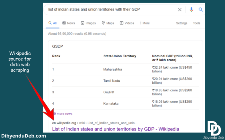
The data source
I will use an authentic website like Wikipedia for open-source data. A data source that has unquestionable authority. If you simply search Google with the search query “Indian states and union territories with their GDP”the first result you will get is from Wikipedia.
Google search result for Indian GDP
Importing the data from website to Power BI desktop
Power BI allows importing data from numerous sources as I have mentioned in the introductory article on Power BI. Among several sources, one is from “Web“.
As you can see in the below figure, you need to select the “Web” from “Get data” option under “Home” tab. Consequently, a new window will open where the URL is to be provided.
Importing data using URL of particular website
If you have already imported the data once from a website, then the address gets stored in “Recent sources“. It will help you to quickly import the data in case you need the data again to import.
“Recent source” of previously used website URL
As you provide the URL, it will first establish a connection to fetch the data. Next, a “Navigator” will open to show you a preview of the data.
See the below screenshot of the Power BI app on my computer; on the left side, all the tables from the web page will be listed. You can click the particular table you are interested and the table preview will be displayed on the right-hand side.
Navigator and table view
Similarly, if you want to get a glimpse of the web view, just click the “Web view“. A web view of the page will be displayed as shown below.
Web view of the page
Transform/load data to Power BI desktop
Now if you are satisfied and found the particular information you are looking for, proceed with the data by clicking “Load” or “Transform". I would suggest going for the transform option as it will enable you to make the necessary changes in the data.
As I have shown the data below before loading it in Power BI. With the help of Power Query,I have made minor changes like changing the column name, replacing the blank rows or replacing the “Null” values, adding necessary columns etc.
I have already described all these operations in data transformation steps here.
Window for data transformation
Once you are satisfied with the table you created, you can load it in Power BI for further processing.
Add table using examples
Another very useful feature is to "Add table using examples". As you can see this option at the bottom left corner of the window in the below screenshot.
Add table using example
This option is very helpful when the tables Power BI automatically shows do not cater to your purpose.
Suppose for the above web page you can see almost all the structured data in table form on the left pane. But you are looking for some information which is scattered on the page and not in a table form.
In that case, if you click the option “Add table using example” you will be provided with a blank table along with the web view as shown in the above image.
Upon clicking the row of the table Power BI provides several options which you can choose from to fill the table. As shown in the above image, some information with no table structure are there to populate the table.
You can also add several columns by clicking on the column header with “*”. Also change column name or later at the data transformation stage.
Final words
So, I hope this article will help you to collect required information from any web page using this feature of Power BI. It is very simple to use only you need to be aware of its existence.
My purpose was to provide you with a practical example of real world data which will make you familiar to this feature. And also to document all the steps for my future reference.
For data analysts and those who just want to get their desired data, writing web scrapers is pure time waste. I myself have written several web scrapers. It obviously has some benefits and can get you some very specific data from several webpages.
But if your data is not scattered in multiple webpages and can be fetched from specific URL, Power BI is your best friend. It will save your lots of time of collecting data and you can straight way jump to the main task of data analysis.
If you find the article helpful, please let me know commenting below. Also if you have any question regarding the topic I would love to discuss with you.
Joining tables is an important feature to combine information from several tables. We can join tables in Power BI desktop with a very nifty merging feature provided with it..
In this article, I am going to demonstrate how to join tables in Power BI desktop with some practical data. The data are all open source. You can collect them from the links provided and use them to practice.
Combining data
When it comes to combining data in tables, it can be done in two ways. One is you may need to increase the rows of a table with new data. This type of data combination is known as “Appending“.
Whereas when you add columns with new information with an existing table, it is called “Merging“.
Power BI provides both of these features under the “Home ” tab (as in the below figure). You need to use them according to your requirement.
Merge and Append queries
This particular article is on joining tables. So we are going to discuss the Merge queries option here only with suitable example.
Lets first discuss different kinds of joins. This will be an overview so that you can make the right decision while selecting join types while merging queries. Also will suggest going through the Microsoft documentation page for details.
The data set
The data set I have used for demonstration purpose is on India’s state-wise crop production collected from data. world. And another data set with India’s state-wise rainfall from different years.
Both the data set presents a real-world experience. The data is collected in raw form and refined using data transformation feature of Power BI. You can go through all the data transformation steps here.
The measures used for different calculations are described in this article.
The first table that is the crop production table contains the area under different crops in hectare (ha) respective to different districts of different Indian states. Whereas the second table i.e. the rainfall table has the rainfall record in mm respective to different districts of Indian states.
Replacing/removing errors
While importing the data from the CSV file or from the web itself, you may face some missing values. When it gets imported in Power BI, the missing values are shown as “Error“.
Now you can not proceed without handling these errors. One way is to replace these errors with proper values. It may be mean or median of rest of the values of particular variable or you can simple remove the rows with missing values.
In the below screenshot you can see how I have replaced the error with a suitable descriptive value. The “Remove errors” option will simply remove the corresponding rows.
Now suppose we want information on both the cropped area as well as rainfall of particular state and districts. Then we need to join the tables with proper conditions.
Different kinds of join tables in power bi desktop
Now Power BI will ask you about the particular join type you are interested to apply. And in order to use the correct join, we should have the idea about different joins. So here is a vivid description with examples of different joins.
For demonstration purpose I have picked few rows from both the tables and created two tables.
Left outer join
It is a prevalent joining process and the default one in Power BI, where the left or 1st table (as in the figure below) retains all of its rows and matching rows from the right or 2nd table. As the text from “Merge queries” option of Power BI displays “All from first, matching from second“.
Suppose we want to know the rainfall of some particular districts with a definite amount of cropped area. So how will you join the two tables to fetch the information? Here is left outer join to help you. See the below figure
Left outer join
In the above figure the particular information we are interested are colored as green cells. The corresponding information has the same color code in the second table.
So, as per the rule of the left outer join, all the rows (yellow coloured) of the left table and the green-coloured rows of the right table has been joined in the new table.
The Venn diagram at the bottom right corner describes the joining process in colour codes. According to this diagram, the matching rows are called the interaction of the two sets. So here the new table consists of the complete left set and the interaction of the sets.
Right outer join
Now suppose we are interested to know the information exactly opposite to what we have fetched earlier. This time we want to know the cropped area of districts having particular rainfall. So, here the right outer join we need to perform.
Right outer join of tables in Power b BI desktop
Full outer join
When we are in need of information of all the states and districts with their cropped area and rainfall, we should go for a full outer join. As the name suggests, this join will return all the records including the matching ones.
Full outer join of tables in Power BI desktop
Here is the final output from the full outer join. The rows contain both the rainfall and cropped area information including the matching rows (in green colour).
Inner join
Again if we need information on the rainfall of those districts with cropped area data as we have nothing to do with rainfall data for those districts not having any cropped area information. In this situation, the inner join produces the desired result.
See the below figure where we have applied inner join on both the tables.
Inner join of tables in Power BI desktop
See in the above image, only the matching rows are kept and all other rows have been excluded.
Left anti join
Suppose for the sake of data analysis, we need only those states and respective districts for which we don’t have any rainfall data, how can we fetch the required information?
Not to worry here the particular join type we need to apply is left anti join. Which will keep all the rows from the left table removing all those which have a match in the right table. See the below example.
Left anti join of tables in Power BI
Here in the above image we just have the required information from the left table of state wise cropped area and everything else have been excluded.
Right anti join
Now suppose we need information exactly opposite the earlier one i.e. we need only the rainfall data of all those districts for which we don’thave any information on the cropped area. The join we will apply here isright anti join.
See the below demonstration with the two tables.
Right anti join of tables in Power BI
In the above figure, the crop production tables have been joined with the rainfall table using the right anti join. You can see that all the rows of rainfall table have been retained excluding the matched rows from the crop production table.
Join tables in Power BI desktop
Now lets see a practical application of joining tables in Power BI desktop.
When you click the merge query option of Power BI desktop, you will see the first table as the active table (the selected able while clicking the merge query option).
You need to select a column from the table with unique values and can act as a key. Then a drop-down will allow to chose from the available tables. Again you have to select another column from the second table using which both the tables can be joined.
Then you need to select the particular join option from the drop-down as shown below. All the join options are available in the same sequence as we discussed above.
Join tables options in Power BI desktop
For example here in the above image, you can see I have selected column “State_name” from the table “India_statewise_crop_production” and the column “SUBDIVISION” from the second table “rainfall_India” as the key columns for joining.
Now our purpose was to keep all the crop production information with matching rainfall data of the corresponding districts. So, I opted for “Left outer join” which is also the default option. You can choose any of them as per your requirement.
Now simply click and see the operation in process.
Selecting rows from the joined table
Now the newly created column will appear in the table. You can see in the below image that the whole table is displayed as a column. So you need to select the particular column and deselect the option “Use original column as prefix“.
See in the above image, by default the complete table appears as row element in the first table. You need to select the particular columns of the table you want here.
Use of advanced editor
Use of advanced editor of Power BI allows more flexibility to change the M script itself yo make desired changes in the output. The M language is at the core of every Power BI application.
See in the below image, the option “Advanced Editor” under the “Home” tab shows the M script behind the particular application. You can tweak them to change the join type or column names etc.
Editing M script for Joining tables in Power BI desktop
Final words
So, here is all about on join tables in Power BI desktop. I have tried to cover all the basics of each kind of join with examples. So that the you can understand the logic behind the joins. And apply the right kind for your need.
Joining tables and fetching the exact information is the core of data modelling. In order to obtain a good visual representation of the Power BI report, a good data modelling is must.
I hope this article will help you to get a good grip on this very fundamental operation of Power BI. If you have queries or doubt, please comment below. I would like to answer them.