Deep learning training process: basic concept

Deep learning training

In this article, we will discuss how deep learning training is conducted for problems like speech recognition, image recognition etc. You will have a basic idea about the training algorithm and how it adjusts the weight to reduce the error. A brief discussion will follow on different components of the training process of a deep learning algorithm.

Deep learning actually a very old concept of Machine Learning but it took a long time to gain popularity. Around 2010 it came to prominence and found many uses in fields like near human-level skills in image recognition, speech recognition, improved machine translation, digital assistants like Siri in apple, google know in android applications, Amazon’s Alexa etc. 

In case you have sufficient data to train the neural network and high capacity GPU then deep learning can be a good choice for its high accuracy. Higher GPU capacity enhances the model performance. 

For problems like speech recognition, the data volume is naturally lesser than image recognition. Data transfer from CPU to GPU plays a significant factor in determining learning efficiency in such smaller problems like speech recognition. But data parameter reduction can not be a solution for problems involving high volume data like image recognition.

Example of Deep learning training

See the following two variables. If we carefully analyse, we can identify that they are related and the relationship between them is Y=2X-1

Human intelligence can identify it by some trial and error methods as long as it is simple like the present one. Deep learning also follows the same principle for identifying the relationship. This process is called learning.

It applies some random values called weights at first to get the output. Initially, the output is much different than the expected one. So, the learning process goes on adjusting the weights and minimize the difference between the estimated and expected output. Thus ultimately it provides an accurate result.

Now if we use these variable combinations in a deep learning network and predict the value of Y corresponding to a value of X=6. It will predict Y= 10.99 instead of 11. As this prediction only on the basis of this sample so, the algorithm is not 100% certain if the prediction is correct.

Role of layers in deep learning training

Deep learning can have tens and thousands of layers theoretically. But when it has a lesser number of layers i.e. only 2-3 layers that learning method often referred to as shallow learning. Let’s consider a deep learning layer has n number of layers. Then if we try to use it for pattern recognition then the consecutive layers will try to identify special features of the pattern. 

The more advance the layer, the more advance feature it will identify. In this fashion, after several rounds of optimization of weights, the final layers will recognize the actual pattern. See the below schematic diagram to understand the process.

Deep learning training for image recognition

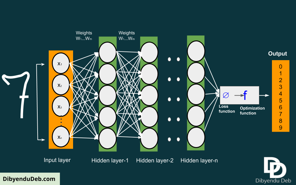
Here what we want the deep learning network to find the digit 7. As you can see we have used n numbers of hidden layers for feature extraction and to identify the character accurately. That’s why this learning process is often referred to as the “multi-stage information distillation process”.

Each hidden layer and input have got some weights, which act as parameters of the layers. After each iteration, we calculate the errors. In the next iteration, the weights again get adjusted to improve the performance further by reducing the error. 

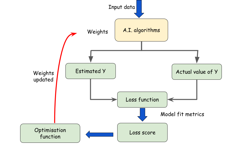
This difference between the estimate and expected output is calculated through a loss function. This loss function in a way represents the goodness of fit of the model using the loss score and help to optimize the weights. See the following diagram to understand the process.

Deep learning training cycle

Some key terms used here are like:

Loss function

This is also known as cost function or objective function and used to calculate the deviation of the estimate from the true value. The probabilistic framework used for this function is maximum likelihood. In the case of classification problem, the loss function is a cross-entropy whereas in case of regression problems the Meas Squared Error (MSE) is generally used.

Weight adjustment

The training process starts with some random values of the weights. Calculated the error with these weights and in next cycles again adjust the weights to further reduce the error. This process continues unless a model with satisfactory performance is achieved.

Batch size

If the problem data set is of large size then for training the model small batches of example data is generally used. Such example data with small batch sizes are very handy for an effective estimation of the error gradient. If the complete data set is not very large, then the batch size can be the whole data set.

Learning rate

The rate at which the weights of the layers are adjusted is called the learning rate. The derivative of the error is used for this purpose.

Epochs

This term indicates the no of cycles of weight adjustment needed to achieve a good enough model with satisfactory accuracy. We need to mention the no of epochs we want the training process should go through beforehand while defining the model.

Such a model has the ability to generalize, which means the model trained in such a fashion that the model performs equally well with an independent data set as it has done during the training. 

So again I would like to mention that the basic idea of deep learning is very simple and rather empiric than theoretical. But this simple training process when scaled sufficiently can appear like magic. 

Backpropagation with Stochastic Gradient Descent

The above figure represents one cycle of the training process through which the weights are adjusted for the next cycle of training. This particular algorithm for training the deep learning network is called the Backpropagation algorithm due to its property of using feedback signal to adjust the weights.

The backpropagation algorithm performs weight optimization through an algorithm known as Stochastic Gradient Descent (SGD). This is the most common algorithm found in almost all neural networks for the optimization process.

Nearly all deep learning is powered by one very important algorithm: Stochastic Gradient Descent (SGD)

Deep Learning, 2016

The iteration of the training process only when a good enough model is found or the model fails to improve or stuck somewhere. Such a training process if often very challenging, time taking and involves complex computations. 

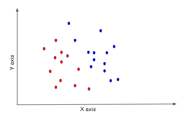
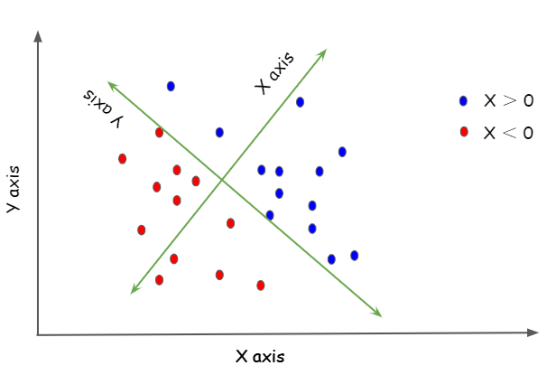
The problem with non-convex optimization

Unlike other Machine Learning or regression modelling process, the deep learning training involves non-convex optimization surface. Where in other modelling processes the error has a space shaped like a bowl with a unique solution

But when the error space is a non-convex one like in case of neural networks, there is neither a unique solution nor any guarantee of global convergence. The error space here comprises of many peaks and valleys with many really good solutions and also with some spurious good estimates of the parameters.

Different steps of training and selecting the best model

A deep learning model performance can be drastically improved if it is trained well. Also scaling up the number of training example and model parameters also play an important role in improving the model fit.  Now we will discuss different steps of training a model.

Cleaning and filtering the data

It is a very important step before you jump to train your model. A data set properly cleaned and filtered is even more important than a fancier algorithm. A data set not cleaned properly can result in a misleading conclusion. 

You must be aware of the phrase “garbage in, garbage out” popularly known as GIGO in software field; which means that wrong or poor quality input will result in faulty output. So, proper data processing is of utmost importance to work a model effectively.

Data set splitting

A model when built, it needs to be tested with an independent data set, which has not been used in model training. If we don’t have such an independent data set, then we need to split the original data into two parts. One is a training data set (generally 70-80% of the total data) and the remaining part of the data as test data.

Train and test data splitting

Tuning the model

Tuning of the model mainly comprises of estimation of two main parameters of any model viz model parameter and Hyperparameter.

Model parameters

Model parameters are those which define an individual model. These parameres are calculated from the training data itself. For example, the regression coefficients are the model parameters which are calculated from the data set on which the model is trained.

Hyperparameter

These parameters are related to the higher structure of the algorithm and decided before the training process starts. Examples of such parameters are like the no of trees in a random forest, in case of regularized regression strength of the penalty used.

Cross-validation score

This is a model performance metric which helps us to tune the model by calculating a reliable estimate of model performance using the training data. The process is simple. We generally divide the data into 10 groups, use the 9 groups out of these to train the model and the rest one to validate the result. 

10-fold cross validation process

And this process will be repeated 10 times with different combinations of train and validation sets of data. That’s why it is generally called 10-fold cross-validation. On completion of all these 10 rounds, the performance of the model is determined by averaging the scores.

Selecting the best model

To select the best performing model, we take the help of a few model comparison metrics like Mean Squared Error (MSE) and Mean Absolute Error (MAE) for a regression problem. The lower the values of MSE and MAE the better is the model. 

Mean Absolute Error(MAE)

If y is the response variable and yis the estimate then MAE is the error between these npair of variables and calculated with this equation:

MAE is a scale-dependent metric that means it has the same unit as the original variables. So, this is not a very reliable statistic when comparing models applied to different series with different units. It measures the mean of the absolute error between the true and estimated values of the same variable. 

Mean Square Error (MSE)

This metric of model comparison is as the name suggests calculate the mean of the squares of the error between true and estimated values. So, the equation is as below:

Whereas in the case of classification problems the common metric that used is Receiver Operating Characteristic (ROC) curve. It is a very important tool to diagnose the performance of MLAs by plotting the true positive rates against the false-positive rates at different threshold levels. The area under ROC curve often called AUROC and it is also a good measure of the predictability of the machine learning algorithms. A higher AUC is an indication of more accurate prediction

Conclusion

At last, a word of caution is to use deep learning wisely for your problem, as it is not suitable for many real-world problems especially when the available data size is not big enough. In fact, deep learning is not the most preferred Machine Learning method used in the industry.

If you are new in the field of Machine Learning, then it is generally a very enticing application of deep learning blindly for any problem. But if there is a different suitable Machine Learning method is available then it is not a wise decision to go for a computation-intensive method like deep learning.

So its a call of the researcher to judge his requirement and available resources to choose the appropriate modelling method. The particular problem, its generic nature and experience in the field play a pivotal role to use the power of deep learning neural network efficiently.

Training a deep learning model is very important to get an accurate result. This article has a detailed discussion on every aspect of this training process. The theoretical background, algorithms used for training and also different steps of it. I hope you will get all your questions related to deep learning training answered here. However please feel free to comment below about the article and also any other questions you want to ask.

References

Artificial intelligence basics and background

Artificial Intelligence basics

Artificial Intelligence (AI) is a buzz word in almost all walks of our life with a meteoric growth recently. For the last few years,  it has come up as a superpower controlling the future of every scientific endeavour. Be it AI-powered self-driving car, disease detection in medical research, image/speech recognition or big data these are just the tips of the iceberg with respect to the enormous possibilities Artificial Intelligence capable of.  This article covers the Artificial intelligence basics with its genesis including modern history.

Artificial intelligence is a broad term encompassing both Machine Learning and Deep Learning. In which Machine Learning is again a bigger domain with the subdomain Deep Learning. These three domains of advance computing can be represented by the following diagram.

Artificial Intelligence basics: Machine Learning and Deep Learning as sub domains

Background of Artificial Intelligence, its genesis

Before we start with the Artificial intelligence basics, we should know its background. The first instance of any machine having some intelligence akin to human was developed by Charles Babbage and English mathematician Lady Ada Lovelace of Victorian England during 1830-40.

It was called a mechanical computer and had the capacity to perform different mathematical computation. The machine algorithm she developed lead to the creation of an early computer which just existed only in paper till then. So, Ada Lovelace, the daughter of famous poet Lord Byron was named the world’s first computer programmer

Turing machine: one step towards modern computer

Another similar example is the Turing Machine developed by Allan Turing in 1950. It can be designated as the first instance of a machine having Artificial Intelligence. He wrote a famous article on Turing Machine titled “Computing Machinery and Intelligence”. 

Turing machine was the first realized model of a computer. Turing invented it while he was working at Cipher school at Bletchley Par and the mission was to break the German Enigma code during the Second World War. It was theoretically similar to modern-day electronic computers. In 1951, the US got its first commercially available electronic stored-program computer named UNIVAC.

The modern history of Artificial Intelligence

After that many years passed with lots of trials and errors, research and development without any significant advancement in the field. The main limitation was lack of training data as images are not abundant at that time and also the computing power also insufficient to analyze the voluminous data. 

However, the scenario took a sharp turn as soon as the advent of computers with higher computational power. The term Artificial Intelligence was first coined in a conference at Dartmouth College, Hanover, New Hampshire in 1956. Again a group of researchers threw themselves to unveil the superpower of AI.

Setbacks

Anyway, critics are always there and their argument against AI now becoming more prominent due to lack of its practical evidence. The government also appeared to be convinced with the argument due to a lack of success in any of the AI projects. As a result funding towards all AI research projects got stopped. It was a big blow and eventually, a winter period started in AI research during 1974 and lasted till 1980

In 1980 the AI research came to the headline for a brief period when the British government showed some interest with an intention to compete with the Japenese advancement in AI research. But that did not last long; soon due to measurable failure of some early-stage computers pushed the field into another prolonged winter period which lasted for long seven years (1987 to 1993).

Breakthrough

But the winning spree of AI was just a matter of time and inevitable. As industry leaders like IBM set foot in the AI industry and took the challenge to show the world what AI is capable of, things start to change. A team of highly qualified scientists and computer programmer threw themselves in this mission and the result was pathbreaking.

Deep Blue: the chess champion supercomputer

The first big success of the AI project was the creation of the supercomputer Deep Blue by IBM. The computer created history when it defeated the then world chess champion, Garry Kasparov on May 3rd, 1997. 

Deep Blue Vs Garry Kasparov
Deep Blue Vs Garry Kasparov (Image source: CBS news, Sunday Morning)

Back then it was so surprising that the reigning champion was not ready to admit that he has lost to a computer with Artificial Intelligence. He was crying foul play and under the suspicion that it was some grandmaster actually playing for the computer.

The computer was so accurate in making the moves but without any human emotions. Where Garry lagged behind being a human. This is where a computer always steps ahead of human being, applying only hard logic based on the vast amount of information fed to it. This victory of Deep Blue over human intelligence ushered a new age of Artificial Intelligence.

Watson: the question-answering AI-based computer

Another historic foot of establishing supremacy over human intelligence achieved by AI in 2011 when a supercomputer named Watson won the famous Quiz show called Jeopardy. In this competition, Watson defeated the defending champions Ken Jennings and Brad Rutter.

Watson and the Jeopardy challenge
Watson and the Jeopardy challenge (Image Source: IBM Research)

Watson is a question-answering computer created by IBM’s DeepQA project in the year 2010 based on Natural Language Processing. Mr David Ferruci of IBM was the key brain behind the idea of Watson. And it got the name after the founder of IBM’s founder and first CEO Thomas J. Watson.

Artificial Intelligence basics

The concept of Artificial Intelligence just reversed the traditional idea of finding a solution for any data-oriented problem. The classical programming or statistical modelling approach usually set the rules first, then apply it on the input data to achieve estimation result. Whereas Artificial Intelligence uses the example answer data along with the input data to learn the rules. See the below schematic diagram to understand it:

Artificial Intelligence basics: Difference between classical programming and AI

This concept of Artificial Intelligence suggests that it gives more emphasis on the hands-on training part. To learn from the data. Indeed this process needs a large amount of data so that the algorithm can be certain about the actual relation between the variables. Thus the idea is to establish the rules more often empirically than theoretically.

The concept of Artificial Intelligence is not a new one though. The concept first came into existence long back in 1950. During its inception, besides the concept of Deep Learning and Machine Learning, it did contain some hardcore programming rule also. For example, playing a chess game back then comprised of a lot of rules programmed to the computer. Such kind of Artificial Intelligence got a name Symbolic AI.

During 1980 the concept of Expert Systems got the limelight across the industries. An expert system on any topic actually provides an interactive information delivery system. Here a machine can play an expert role and based on the user’s input provides suitable information. In the process of developing such expert systems, the Symbolic AI transformed into Machine Learning.

Components of Artificial Intelligence

This has three main components as shown in the above figure:

Input data:

This is very obvious and also common in traditional programming or statistical modelling. We need to feed the input data in order to arrive with the estimation. The sample data in our hand either labelled or non-labelled plays this role as input data. 

Labelled data:

This is the unique part in case of Artificial Intelligence. We need to provide some example answer data to train the programme. The larger the example answer data, the more accurate is the training. This example data set is the labelled data here. As both the variables feature and label are present here. We expect the algorithm will learn from this example and identify the relationship between them.

Error optimization:

This is the third important component which calibrates the algorithm identifying how close is the estimation to the actual value. There are several metrics which provide a good measure of how good the model is performing.

Algorithm to represent the input data

In nutshell, this is the main essence of Artificial Intelligence. All machine learning or deep learning algorithms try to find out some effective way to represent the input data. This representation is of utmost importance as this is the key for successful prediction. 

For example when the problem in hand is to identify any image and the image has colour composition Red, Green and blue; then a very effective way to represent the image can be to identify the number of pixels with red colour. In similar fashion in case of speech recognition, if the algorithm can represent the language and voice modulation effectively the accuracy of recognition gets much higher.

An example of data representation

Here is an example of this representation problem with an easy graphical classification problem. This example I have read in the book “Deep learning with Python” by Keras creator and Google AI researcher Francois Chollet. It is a great book to start your journey with Artificial Intelligence.

Separating the different colour dots using data transformation

See in the above figure the scattered points with two colour groups red and blue. The problem is to find out some rule to classify these two groups. A good solution to this representation problem is to create a new coordinate like the below figure. Now after the change in coordinates, the different colour dots can be easily classified with a simple rule which is the dots are blue when X>0 and red when X<0.

Data representation changing coordinates

AI algorithms: not creative but effective 

This types of transformations are handled by Artificial Intelligence algorithms automatically. Like this coordinate change, other transformations like linear transformation, nonlinear operations, etc. all frequently used functions and are available for Artificial Intelligence algorithms to choose from a predefined space called Hypothetical space. In this sense Artificial Intelligence algorithms are not very creative, all they do is to select functions from this space of possibilities.

Although the algorithm is not creative, often does the work. The algorithm takes the input data; then applies suitable transformation from the Hypothetical space; the algorithm takes the help of the feedback signal obtained from the output and expected output and with this guidance, attempt to represent the input data.

The following diagram represents the flow of information process for ease of understanding.

Artificial Intelligence basics: Schematic of AI algorithm functioning

Final words

So, in the simplest terms, Artificial Intelligence is all about learning through trials and examples. You provide lots and lots of example answers and the algorithm will go on perfecting itself. Unlike other prediction algorithms which reaches a plateau after a certain number of trails, AI algorithms keep improving.

A good practical example such learning process is Google’s Quick Draw. It is an AI-driven drawing game hosted by Google. As claimed by Google, it is the world’s largest doodling data set and you can also your drawing sample to it.

A screenshot of Google’s Quick Draw

It is an experimental research on the use of AI. You will surprise to see how effortless and quick the drawing it offers using AI. You can draw a picture in less than 20 seconds time! And the reason behind its so high accuracy in pattern recognition is again as I mentioned, a huge database of example answers. Almost 15 million people have uploaded more than 50 million drawings in the database.  

Not only drawing it is the collection of several other experiments with music, video, natural language processing and many more with open access code. You can try the codes as they are open-sourced and also add your own code of AI application.

Expectations from AI should be rational and for Long term

One problem with Artificial Intelligence was the possibilities were always hyped out of proportions. The goals and expectations were set for a too short term. The obvious result of which was disappointment and loss in interest. Such disappointment resulted in two winter period in AI research as I have mentioned before.

Such winter periods slow down the development process for years together and not at all good for the researchers and scientists putting tremendous effort in AI research. They become the victims of the irrational hype created by press and media and some over enthusiasts.

When the dreams got shattered all research projects experience a crunch in research funding. The scientists who may be at the verge of some significant result got stuck with their research just because of insufficient fund. This is very heartbreaking and may deprive a scientist of his life long research achievements.

Many of the expectations from AI technology during 1960-70 are still far-reaching possibilities even in 2020. Similarly, the hype with AI in recent years may be an exaggeration too and may lead to another winter period.

Conclusion

So, we need to be very cautious in making realistic expectations out of AI. Instead of setting short term goals, we should look for a long term broad objective. Should give the researchers sufficient time to proceed with their research and development activities.

There is no denying that AI is going to be our everyday best friend. It is going to make our lives much much easier in the coming days. The day is not very far when we will take help of AI in every problem we face, we will take suggestion when we will feel sick, it will help to educate our kids, take us to our destination, help us to understand a foreign language and in doing so AI will take the whole humanity to a newer level of evolution.

This is not an unrealistic expectation and the day will eventually come. We just need to keep patience and have faith on highly talented AI scientists working hard to make this dream a real one.

References

Comparing machine learning models for a regression problem

Comparing regression models

Comparing different machine learning models for a regression problem is necessary to find out which model is the most efficient and provide the most accurate result. There are many test criteria to compare the models. In this article, we will take a regression problem, fit different popular regression models and select the best one of them. 

We have discussed how to compare different machine learning problems when we have a classification problem in hand (the article is here). That means in such cases the response variable is a categorical one. Different popular classification algorithms are compared to come out with the best algorithm. 

NB: Being a non-native English speaker, I always take extra care to proofread my articles with Grammarly. It is the best grammar and spellchecker available online. Read here my review of using Grammarly for more than two years. 

Comparing regression models

So, what if the response variable is a continuous one and not categorical. This is a problem of regression then and we have to use regression models to estimate the predicted values. In this case also several candidate regression models. Our task is to find the one which serves our purpose. 

So, in this article, we are taking a regression problem of predicting the value of a continuous variable. We will compare several regression models, compare their performance calculating the prediction accuracy and several goodnesses of fit statistics. 

Here I have used five most prominent and popular regression models and compared them according to their prediction accuracy. The supervised models used here are

The models were compared using two very popular model comparison metrics namely Mean Absolute Error(MAE) and Mean Square Error (MSE). The expressions for these two metrics are as below:

Mean Absolute Error(MAE)

Comparing different machine learning models for a regression problem involves an important part of comparing original and estimated values. If \dpi{150} y is the response variable and \dpi{150} \widehat{y} is the estimate then MAE is the error between these \dpi{150} n pair of variables and calculated with this equation:

MAE is a scale-dependent metric that means it has the same unit as the original variables. So, this is not a very reliable statistic when comparing models applied to different series with different units. It measures the mean of the absolute error between the true and estimated values of the same variable. 

Mean Square Error (MSE)

This metric of model comparison is as the name suggests calculate the mean of the squares of the error between true and estimated values. So, the equation is as below:

Python code for comparing the models

So, now the comparison between different machine learning models is conducted using python. We will see step by step application of all the models and how their performance can be compared.

Loading required libraries

All the required libraries are first loaded here.

import numpy as np # linear algebra
import pandas as pd # data processing
from sklearn.linear_model import LinearRegression
from sklearn.preprocessing import PolynomialFeatures
from sklearn import metrics
from pandas import DataFrame,Series
from sklearn.tree import DecisionTreeRegressor
from sklearn.ensemble import RandomForestRegressor
import matplotlib
import matplotlib.pyplot as plt
from sklearn import linear_model
from sklearn.model_selection import train_test_split,cross_val_score, cross_val_predict
import missingno as msno # plotting missing data
import seaborn as sns # plotting library
from sklearn import svm

The example data and its preprocessing

The data set used here is the car data set from Github and you can access the data file from this link. The data set has the following independent variables:

  • Age
  • Gender
  • Average miles driven per day
  • Personal debt and
  • Monthly income

Based on these independent variables we have to predict the potential sale value of a car. So, here the response variable is the sale value of the car and it is a continuous variable. That is why the problem in hand is a regression problem.

Importing the data

The below piece of code will use the panda library read() function to import the data set into the working space. The describe() function is for a brief idea about the data.

dataset = pd.read_csv("cars.csv")
dataset.describe()

Displaying the last few columns of the data set to have a glimpse of the data and variables.

Last few columns of the data set

Check the data for missing values

The following code is to check if there any missing value in the data set. Missing value creates a problem in the analysis process. So, we should filter these values in the data pre-processing stage. Here we will find out which columns contain missing values and the corresponding rows will be simply dropped from the data set.

# Finding all the columns with NULL values
dataset.isna().sum()
# Drop the rows with missing values
dataset = dataset.dropna()

Creating basic plots with the data

Here we create the joint distribution plot of the independent variables

sns.pairplot(dataset[['age', 'miles', 'debt', 'income', 'sales']], diag_kind="kde")
Joint distribution plot of the  independent variables
Joint distribution plot of the independent variables

Splitting the data set

Data splitting is required to create training and testing data sets from the same car data. I have taken 80% of the whole data set as training data and the rest 20% of data as the test data set. The following python code is for this splitting purpose.

train_dataset = dataset.sample(frac=0.8,random_state=0)
test_dataset = dataset.drop(train_dataset.index)

Normalizing the training data set

First of all we will see the summary statistics of all the variables using the describe() function of sklearn library.

# Calculating basic statistics with the train data
train_stats = train_dataset.describe()
train_stats.pop("sales") # excluding the dependent variable
train_stats = train_stats.transpose()
train_stats

Here from the below stats about the data set, we can see that different variables in the data set has very large range and deviations, which may create problem during model fitting. So, before we use this variables in model building process, we will normalize the variables.

Summary statistics of the  training data set
Summary statistics of the training data set

Creating a function for normalization

Using the mean and standard deviation of each of the variables, we will convert them into standard normal variates. For that purpose, we will create the function as in below.

# Creating the normalizing function with mean and standard deviation
def norm(x):
  return (x - train_stats['mean']) / train_stats['std']
normed_train_data = norm(train_dataset)
normed_test_data = norm(test_dataset)

Separating the response variable and creating other variables

Now a most important step to store the response variable in a separate variable.

train_labels = train_dataset.pop("sales") # using .pop function to store only the dependent variable
test_labels = test_dataset.pop("sales")
x_train=normed_train_data
x_test=normed_test_data
y_train=train_labels
y_test=test_labels

As we are now finished with the data pre-processing stage, we will start with the modelling steps. So, let’s start coding for all the five models I have mentioned to predict the car sale price.

Application of Multiple Linear Regression

First of all Multiple Linear Regression (MLR). This simple linear regression only but we will include all the independent variables to estimate the car sale price. The LinearRegression() function from LinearModel module of sklearn library has been used here for the purpose.

lin_reg = LinearRegression()
lin_reg.fit(x_train,y_train)
#Prediction using test set 
y_pred = lin_reg.predict(x_test)
mae=metrics.mean_absolute_error(y_test, y_pred)
mse=metrics.mean_squared_error(y_test, y_pred)
# Printing the metrics
print('R2 square:',metrics.r2_score(y_test, y_pred))
print('MAE: ', mae)
print('MSE: ', mse)
Metrics for MLR

Application of Decision Tree regression

dt_regressor = DecisionTreeRegressor(random_state = 0)
dt_regressor.fit(x_train,y_train)
#Predicting using test set 
y_pred = dt_regressor.predict(x_test)
mae=metrics.mean_absolute_error(y_test, y_pred)
mse=metrics.mean_squared_error(y_test, y_pred)
# Printing the metrics
print('Suppport Vector Regression Accuracy: ', dt_regressor.score(x_test,y_test))
print('R2 square:',metrics.r2_score(y_test, y_pred))
print('MAE: ', mae)
print('MSE: ', mse)
Metrics for Decision tree

Application of Random Forest Regression

rf_regressor = RandomForestRegressor(n_estimators = 300 ,  random_state = 0)
rf_regressor.fit(x_train,y_train)
#Predicting the SalePrices using test set 
y_pred = rf_regressor.predict(x_test)
mae=metrics.mean_absolute_error(y_test, y_pred)
mse=metrics.mean_squared_error(y_test, y_pred)
# Printing the metrics
print('Suppport Vector Regression Accuracy: ', rf_regressor.score(x_test,y_test))
print('R2 square:',metrics.r2_score(y_test, y_pred))
print('MAE: ', mae)
print('MSE: ', mse)
Metrics for Random Forest regression

Application of Support Vector Regression

from sklearn.svm import SVR
regressor= SVR(kernel='rbf')
regressor.fit(x_train,y_train)
y_pred_svm=regressor.predict(x_test)
#y_pred_svm = cross_val_predict(regressor, x, y)
mae=metrics.mean_absolute_error(y_test, y_pred_svm)
mse=metrics.mean_squared_error(y_test, y_pred_svm)
# Printing the metrics
print('Suppport Vector Regression Accuracy: ', regressor.score(x_test,y_test))
print('R2 square:',metrics.r2_score(y_test, y_pred_svm))
print('MAE: ', mae)
print('MSE: ', mse)
Metrics for Support Vector Regression

Application of Deep Learning using Keras library

Here is the deep learning model mentioned. A sequential model has been used. The model has been created as a function named build_model so that we can call it anytime it is required in the process. The model has two connected hidden layers with a Rectified Linear Unit (relu) function and an output layer with a linear function.

The hidden layers have 12 and 8 neurons respectively with all the 8 input variables. Mean Squared Error is the loss function here as it is the most common loss function in case of regression problems.

def build_model():
  model = keras.Sequential([
    layers.Dense(12,kernel_initializer='normal', activation='relu', input_shape=[len(train_dataset.keys())]),
    layers.Dense(8, activation='relu'),
    layers.Dense(1, activation='linear')
  ])

  optimizer = tf.keras.optimizers.RMSprop(0.001)

  model.compile(loss='mse',
                optimizer=optimizer,
                metrics=['mae', 'mse'])
  return model
model = build_model()

Displaying the model summary

This part of code is to show the summary of model we built. All the specifications mentioned above has been shown in the below screenshot of the output.

model.summary()
Deep learning  model summary
Deep learning model summary

Training the model

We have used 10 rows of the training data set to check the model performance. As the result seems satisfactory so, we will proceed with the same model.

example_batch = normed_train_data[:10]
example_result = model.predict(example_batch)
example_result

Fitting the model

Now we will fit the model with 1000 epochs and store the model training and validation accuracy in the object named history.

EPOCHS = 1000

history = model.fit(
  normed_train_data, train_labels,
  epochs=EPOCHS, validation_split = 0.2, verbose=0,
  callbacks=[tfdocs.modeling.EpochDots()])
History of the model fit

Here we will produce a glimpse of the history stats to understand how the training process progresses.

hist = pd.DataFrame(history.history)
hist['epoch'] = history.epoch
hist.tail()

Plotting the MAE score during the training process

As we are using 1000 epochs to train the model. It necessarily suggests that there are 1000 forward and backward passes while the model is trained. And we expect that with each passes the the loss will decrease and model’s prediction accuracy will increase as the training process progresses.

plotter = tfdocs.plots.HistoryPlotter(smoothing_std=2)
plotter.plot({'Basic': history}, metric = "mae")
plt.ylim([0, 10000])
plt.ylabel('MAE [sales]')

In the above plot, we can see that both the training and validation loss decreases in a exponential fashion with the increase in number of epochs.

test_predictions = model.predict(normed_test_data).flatten()
a = plt.axes(aspect='equal')
plt.scatter(test_labels, test_predictions)
plt.xlabel('True Values [sales]')
plt.ylabel('Predictions [sales]')
lims = [0, 40000]
plt.xlim(lims)
plt.ylim(lims)
_ = plt.plot(lims, lims)

Plotting the result

Here we have plotted the predicted sale prices against the true sale prices. And from the plot it is clear that the estimate is quite close to the original one.

Original Vs predicted values of sale price of cars

Plotting the error

error = test_predictions - test_labels
plt.hist(error, bins = 125)
plt.xlabel("Prediction Error [Average_Fruit_fly_population]")
_ = plt.ylabel("Count")

Here we have plotted the error. Although the distribution of error is not a true Gaussian, but as the sample size increases, we can expect it will tend to a Gaussian distribution.

mae=metrics.mean_absolute_error(test_labels, test_predictions)
mse=metrics.mean_squared_error(test_labels, test_predictions)
# Printing the metrics
#print('Suppport Vector Regression Accuracy: ', lin_reg_pl.score(x_poly,y_train))
print('R2 square:',metrics.r2_score(test_labels, test_predictions))
print('MAE: ', mae)
print('MSE: ', mse)
Metrics of Deep learning models

Conclusion

So, here we can compare the performance of all the models using the metrics calculated. Let’s see all the models used to predict the car sale price together along with the metrics for the ease of comparison.

Model typeMAER Square
MLR28210.80
Decision Tree22110.84
Random Forest18170.88
Support Vector Machine72320
Deep learning/ANN27860.8
Comparison table for all the models used

From the table above, it is clear that for the present problem, the best performing model is Random Forest with the highest R square (Coefficient of Determination) and least MAE. But we have to keep in mind that the deep learning is also not far behind with respect to the metrics. And the beauty of deep learning is that with the increase in the training sample size, the accuracy of the model also increases.

Whereas in case of other models after a certain phase it attains a plateau in terms of model prediction accuracy. Even increasing training sample size also can not further improve the model’s performance. So, although deep learning occupies the third position in present situation, it has the potential to improve itself further if availability of training data is not a constrain.

If the data set is small and we need a good prediction for the response variable as the case here; it is a good idea to go for models like Random Forest or Decision tree. As they are capable of generating good prediction with lesser training data or labelled data.

So, finally it is the call of the researcher or modeler to select the best suited model judging his situation and field of knowledge. As different fields of science generate experimental data with distinct nature and a very good model of another field may fail completely to predict.

References

What is deep learning? an overview

Deep learning basics

Deep learning is actually an artificial intelligence function with immense capability to find out the hidden pattern within a huge amount of data generated in this era of data explosion. It is an advanced learning system which mimics the working principle of the human brain. Such kind of vast unstructured data is not possible for the human being to analyze and draw some conclusion. So, such a learning procedure has been proved very helpful to make use of big data.

According to Andrew NG the founder of deeplearning.ai and popular Coursera deep learning specialist

Deep learning is a superpower. With it you can make your computer see, synthesize novel art, translate languages, render a medical diagnosis, or build pieces of a car that can drive itself. If that is not a superpower, I don’t know what is.

Andrew NG

In this respect, machine learning is a much bigger domain and deep learning can be considered as a subdomain of it. Deep learning relates to the deep neural network and mainly works in an unsupervised manner.  The network is popular with the name Artificial Neural Network as it mimics our brains vast network of neurons.

Deep-Neural-Network
A schematic diagram of neural network with two hidden layer

Difference between machine learning and deep learning

 The main difference between these two processes lies in the feature extraction process from images. Feature extraction is the basic component of both the processes.

Feature extraction

But the difference is machine learning requires to perform this process manually and then feed this information in the model. Whereas in deep learning the feature extraction happens automatically and provided to the network to match with the object of interest. In this context, deep learning is called an “end-to-end” process of learning.  

Resource intensive

Another major difference between these two processes is data processing capability. Deep learning can make good use of a huge number of labelled data provided you have sophisticated Graphics Processing Unit (GPU). On the other hand, machine learning has different modelling techniques to give you a good estimate even with a less number of labelled data. 

Scaling with the data

Deep learning has a big plus point over machine learning which makes deep learning far more accurate than machine learning is that deep learning algorithm scales itself with the data. That means as we use more images to train the deep learning algorithm it will give the more accurate result.

But it is not the case with machine learning algorithms. Machine learning algorithms attain a plateau after a certain level of performance achieved. It will not improve even with more training after this level. See the below image to realize the difference.

Deep learning  improves as the data size increases
Deep learning improves as the data size increases

So, now the question is which approach should be used by one? To answer that I would suggest that it depends on your situation i.e. the type of problem you desire to solve, the GPU capacity available to you and the most important factor how much labelled data you have to train the algorithm.

Deep learning is more accurate than machine learning but more complex too. So unless you have thousands of images to train it and high-performance GPU to process such a large amount of data, you should use any machine learning algorithm or combination of them.

Deep learning: the working principle

Deep learning mainly relies on Artificial Neural Network (ANN) to unravel the wealth of information from big data. So, it is very interesting to know how does this process is actually performed. 

If you have a little exposure to the traditional modelling process, you may have an idea that conventional regression models suffer from various limitations and had to fulfil several assumptions.

And most of the cases it performs not so well in capturing the real nonlinear nature of real-world data. This is mainly because of the traditional regression way of modelling does not attempt to learn from the data. This learning process which makes the real difference between these two approaches. 

The term deep in deep learning suggests the mechanism of information processing through several layers. Deep learning or deep structured learning is mainly based on a learning process which is called representation learning. It is actually finding out representations for hidden feature or pattern recognition from raw unstructured data.

Accuracy of both the approaches

The accuracy deep learning attains in its estimation is impeccable. The applications mentioned above needs to be very precise to satisfy end user’s expectation. And such accuracy can only be provided by deep learning. To achieve such accuracy, it trains itself using the labelled data to continuously improve the prediction by minimizing error. 

So, the amount of labeled data is an important factor determining how perfect is the learning process. For example to make a perfect self-driving car we need to train the algorithm with a huge amount of labeled data like images and videos of road, traffic, people walking on the road or a busy road at any time. 

No doubt deep learning is a very computation-intensive process. Processing such a huge amount of image and videos and then using them to train the algorithm may take days and weeks altogether. 

This was one of the key factors that in spite of the concept of deep learning came back in 1980 it was not in much use till recently. It is just because back then researchers were not equipped with systems with high computing capacity. In today’s era of supercomputers or systems with high-performance GPUs, advanced cloud computing facilities have made processing such enormous size of data possible within hours or even less. 

ANN: mimicking the human brain

Artificial Neural Network or ANN as the name suggests it mimics our brains working principle. In our brain, the neurons are the working unit. The network between the innumerable neurons works as layers in carrying the sensation from different body parts to the designated part of the human brain. As a result, we can feel touch, smell the fragrance, taste a tasty food or hear music.

The learning process

Human being basically learns from past experience. Since childhood, a person gathers experience about everything in his surrounding and thus learn about them. For example, how can we able to identify a dog or cat? Perhaps because we have seen a lot of these animals and learned the differences between their appearances. So, now for us chance of making a mistake in identifying these animals is almost nil.

Deep learning for feature extraction

This is the very nature of the learning process of a human being. The first time a baby sees a dog he/she knows it is a dog from the parents. Gradually through this process, the baby comes to know animals of this appearance are called dogs. This learning process of a human being is exactly followed in case of deep learning. And the result gets more and more accurate as the learning process continues.

ANN also comprises of neurons and the nodes are connected to form a web-like structure. There can be multiple layers of such neurons (generally two to three but theoretically it can be any number). These layers pass different information from one layer to another and finally produces the result.

One layer of neuron act as the input layer for the immediate next neuron layer. The term “deep” actually signifies the number of layers only in any ANN. The most common and frequently used deep learning network is known as a Convolutional Neural Network (ConvNet/CNN).

Convolutional Neural Network (CNN)

CNN is one popular form of deep learning. It actually eliminates the need for manual feature extraction from any image in order to recognize it. CNN used thousands of images and used hundreds of hidden layers for its feature extraction to match it with the object of interest.

The hidden layers are arranged in such a fashion to recognize features with a higher order of complexity. That means the first hidden layer may recognize only the edges of the image whereas the last one will recognize a more complex shape of the image which we desire to recognize.

Applications of deep learning

Today’s digital era is collecting and generating data at every moment of our presence in the digital world. Be it social networking sites, online shopping, online movies or online study/research anything. We are providing lots of data as input to get the desired output from the internet. 

The data size is enormous and also completely unstructured but has a lot of information on it. Which if analyzed properly can help the government to take better policy decision or business houses to frame an effective business plan.

Since last few years, this learning process has been the key concept behind some revolutionary ideas and applications like:

Image colourization

Recently some of the old black & white movies are relaunched with colour effects. If you watch them you may be surprised by the precision and accuracy of the colourization process. Artificial intelligence has made this task possible to complete within a few hours. It was previously only possible with human skills and hard labour.

The famous movie “Pather Panchali” of the Oscar-winning film director Shri Satyajit Ray was shot in black & white. Recently Mr Ankit Bera, Assistant Research Professor of AI at the University of Maryland in U.S. has done an experiment to colourize the movie and the result is really impressive (read the full story here). Here is a comparison of two still frames side by side from the movie for your comparison.

A screenshot from the report

Self-driving car

A self-driving car where deep learning enables a car to recognize a stop sign or to distinguish a pedestrian from a lamppost, judges the situation of a busy road and thus reducing the chance of an accident.

An autonomous car is able to take human-like decisions on the basis every probable situations you may face while driving. It is still in the testing phase. It improves its perfection as it gets trained with more data of real-life traffic condition.

Facial recognition

Its presence is now everywhere, be it biometric attendance system, AADHAR enabled transaction or your mobile’s face lock system. This recognition system is so smart that it identifies you even when you have shaved off your mustache or changed your hairstyle.

Natural language processing and Virtual assistants

In natural language processing, speech recognition where deep learning plays a crucial role in following the command given by a person to his smartphone or any smart device. You may also have tried Google’s speech to text tool to save yourself from typing a lot, so thanks to voice recognition also a gift of deep learning.

Different online service providers have launced several virtual assistants mainly on the basis of this concept. You must have heard the names of apple’s Siri, Microsoft’s Cortana, Amazon’s Alexa etc. all are very popular virtual assistants making our daily lives a lot easier.

Language translations

In language translations deep learning has played a big role as in natural language processing. This has benefitted the travelers, business people and many others who need to visit a lots of place and also communicate a lot with people speaking foreign language.

Chatbots

You may have experienced that in recent times whenever you want to contact the customer support or product help of any company to get some questions answered related to any of their product, the first basic question-answer part is generally automated and intelligently replied without any human interventions.

In medical research

It plays a pivotal role nowadays. In cancer research identifying the affected cells. A dedicated team of researchers at UCLA has built an advanced microscope which used deep learning to pinpoint the cancerous cells.

Many industries like drug industries, automobiles, agriculture sector, board game making brands, medical image analysis are actively conducting research with deep learning in their R&D sector. 

Conclusion

So, I think in this article I am able to give you a basic idea about what is deep learning and how it works. Although the idea of deep learning was conceptualized long back in 1986 due to limitation of resources it did not take up. And took more than a decade to come into action. Today we have sophisticated computing devices and no dearth of data. In fact, there are oceans of data with every aspect of our daily life.

Every moment of our life, our life and every activity happening in the world is getting stored in one or other format of data, mainly as images, videos, audios etc. These data is so huge that conventional process of data analysis can not handle it and simple human capacity would take decades to analyze it.

Here comes deep learning with its fascinating power of data analysis mainly pattern recognition. Deep learning works especially with more accuracy when the database is a large number of audio, video or image files, so it is the best fit for the situation. And this is the reason it gets its name as “Deep” as many features of the images get extracted at different layers of the deep learning process. So, deep actually refers to the depth of layers.

Deep learning is vast topic and a single article can not cover all of its aspects. So its basic features are mainly discussed here and you can start your deep learning process with this article.

Follow this blog regularly as many interesting articles regarding deep learning and its application will be posted here regularly. If you have any particular topic in your mind please let me know by commenting below. Also, share your opinion about this article and how it can be improved further.

References