The evolution of deep learning has experienced many ups and downs since the last few decades. One time it rose to the pick of the popularity, expectations were high and suddenly some setbacks in experimental trials created a loss of confidence and disappointments. This article will cover this journey of deep learning neural network from its inception to its recent overwhelming popularity.
Background of Machine learning
This all started with very basic concepts of probabilistic modelling. These are very elementary statistical concepts from the school syllabus. This was the time even before the invention of the term machine learning. All models, functions were solely crafted by the human mind.
Probabilistic models
These models are the first step towards the evolution of deep learning. These models are developed keeping in mind real-world problems. Variables having relationships between them. Combinations of dependent and independent variables were used as inputs to these functions. These models are based on extensive mathematical theory and more empirical than practical.
Some popular such probabilistic models are as below:
Naive-Bayes classification
It is basically the Bayes theorem with some naive assumption hence the name. The concept of this modelling was established long back during the 18th century. The assumption here is “all the features in the input data are all independent”.
For example, suppose a data set has the data of some persons with or without diabetes disease and their corresponding sex, height and age. Now the Naive Bayes will assume that there is no correlation between all the features between sex, height and age and they contribute independently towards the disease. This assumption is called class conditional independence.
So how this assumption helps us to calculate the probability? Suppose, there is a hypothesis H which can be true or false and this hypothesis gets affected by an event e. We are interested to calculate the probability of the hypothesis being true given that the event is observed. So, we need to calculate: P(H|e)
According to Naive Bayes’ theorem
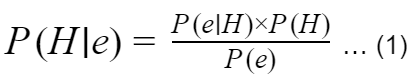
Here, P(H|e) is called the posterior probability of the hypothesis with the information of event e and can not be easily computed. So, we need to break down it as in equation 1. Now we can calculate each of the probabilities separately from the frequency table and calculate the posterior probability.
You can read the whole process of calculation here.
P(H) is the prior probability of the hypothesis before observing the event.
Logistic regression
This regression modelling technique is so basic and popular for almost all classification problems that it can be considered as the “Hello World” of Machine Learning. Yes, you have read it right. It is a process for classification problems. Don’t let the word regression in the name misguide you.
It is originally a regression process which becomes a classification process when the process involves a decision threshold for the prediction. Deciding a threshold for the classification process is very important and tricky one too.
We need to decide the decision threshold depending on the particular case in hand. There can be four types of responses in case of classification problems which are “true positive”, “true negative”, “false positive” and “false negative” (read details about them here). We have to fix the probability of one type of occurrence while reducing another depending on its severity.
Example and basic concept
For example, take the case for a severe crime and it is to decide if the person should be hanged or not. It is a problem of binary classification with two outputs guilty or not guilty. Here the true positive case is the person found guilty when he actually has committed the crime. On the other hand, the true negative is the person found guilty when he has not committed the crime.
So, no doubt the true negative case here is of very serious type and should be avoided at any cost. Hence while fixing the decision threshold, you should try to reduce the probability of true negative while fixing the probability of true positive cases.
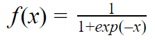
Unlike linear regression predicting the response of a continuous variable, in logistic regression, we predict the positive outcome of a binary response variable. Unlike linear regression which follows a linear function, a logistic regression has a sigmoid function.
The equation for logistic regression:
Initial stages of evolution of Deep Learning
Although the theoretical model of deep learning came in 1943 by Walter Pitts, a logician and Warren McCulloch, a neuroscientist. The model was called McCulloch-Pitts neurons and still regarded as a fundamental study on deep learning.
The first evidence of the use of neural networks in some toys for children made during the 1950s. The same year the legendary mathematician Alan Turing proposed the concept of Machine Learning and even gave hints about the genetic algorithm in his famous paper “Computing machinery and intelligence”.

In 1952, Arthur Samuel first time coined the term Machine Learning. He is known as the father of machine learning. He with his association with IBM also developed the first machine learning programme.
“The perceptron: the perceiving and recognizing automaton” a research paper published in the year 1957 by Frank Rosenblatt set the foundation of Deep Learning network.
In 1965 mathematician Alexey Ivakgnenko and V.G. Lapa arguably developed the first working deep learning network. Ivakgnenko for this contribution is considered as the father of deep learning by many.
The first winter period
The period between 1974-80 is considered as the first winter period. It is a long rough period faced by AI research. A critical report submitted by Professor Sir James Lighthill on AI research as asked by UK parliament played a major role to initiate this period.
The report was very critical about the AI research in the United Kingdom and was in the opinion that nothing has been done in the name of AI research. All expectations about AI and deep learning were all hype; creation of a robot was nothing but a mirage; such comments were very disappointing and resulted in the /retraction of research funding for most of the AI research.
Invention of Backpropagation algorithm
Then in during 1980, the famous Backpropagation algorithm with Stochastic Gradient Descent (SGD) was invented for training the neural network. This can be considered as path-breaking discovery as far as deep learning is concerned. These algorithms are still the most popular among deep learning enthusiasts. This algorithm only led to the first successful application of Neural Network.
LeNet
Come in 1989 we got to see the first real-life application of Neural Net. It was Yann LeCun who made this possible through his tireless effort in Bell Labs to combine the ideas of Backpropagation and Convolutional neural network.

The network was named after LeCun as LeNet. It found its first real-world problem-solving use in identification of handwritten codes. It was so efficient in identifying the codes that United States Postal Service adopted this technology in 1990 for identifying the digits of ZIP codes on the mail envelopes.
Yet another winter period; however brief one
In spite of the success achieved by LeNet, in the same year 1990, the advent of Support Vector Machine pushed the Neural Network almost extinction. It gained very fast popularity mainly because of its easy interpretability and state of the art performance.
It was also a technology came out of from the famous Bell Labs. Vladimir Vapnik and Corinna Cortes pioneered its invention. They started working on it long back in 1963. It’s their continuing effort that resulted in the revolutionized Support Vector Machine of 1990.
Support Vector Machine: a new player in the field
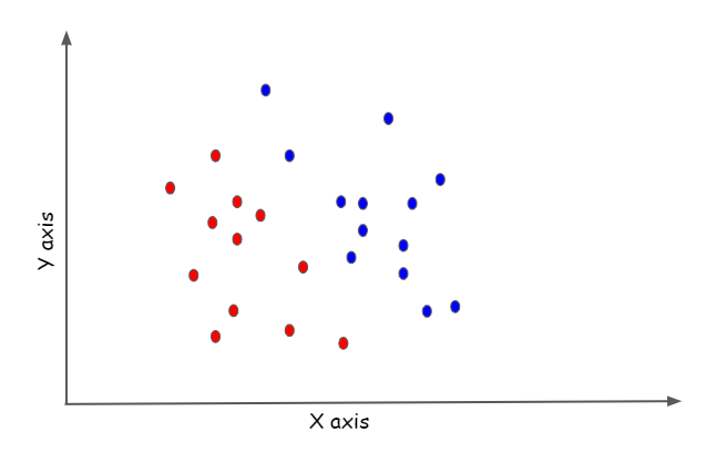
This new modelling is mainly conceptualized on a kernel trick to calculate the decision boundary between two class of variables. Except for a few cases, it is very difficult to discriminate variables on a two-dimensional. It becomes far easier to understand in a higher-dimensional space. A hyperplane of higher dimensional space becomes a hyper line in two-dimensional space i.e. a straight line. This process of transforming the mode of representation is known as kernel trick.
Below is an example of what I mean to say by higher dimension representation for classification.
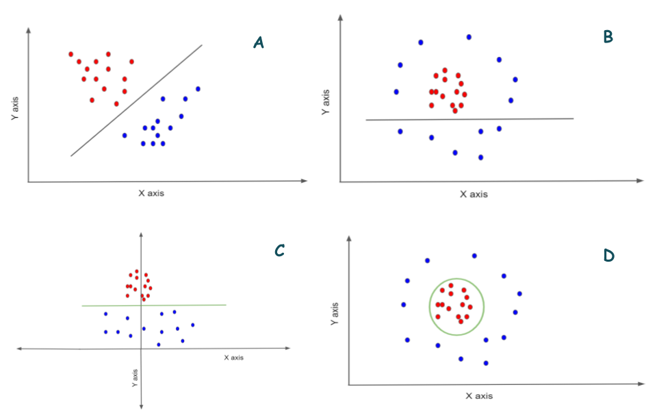
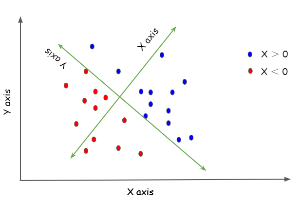
In figure A, two classes of observations that are red and blue classes are classified using a hyperline. It is a straight forward case and the classification is easy. But consider the figure in B here a straight line can not classify the points.
As a new third axis has been introduced in figure C, we can see that the classes are now can be easily separated here. Now how it will look if the figure we again convert it to its two-dimensional version? see the figure in D.
So, a curved hyperline has now separated the classes very effectively. This is what a support vector machine does. It finds a hyperplane to classify the points and then any new point gets its class depending on which side of the hyperplane it resides.
Kernel trick
A kernel trick can be explained as a technique to maximize the margin between the hyperplane and the closest data points. It makes the process very easy by curtailing the need to calculate the new coordinates in the new representation space. The kernel function only calculates the distance between the pair of points.
This kernel function is not something that SVM learns from the data. It is solely crafted by the human mind. The distance between the points in the original space to that of in the new representation space is mapped. And then the hyperplane is created through learning from the data.
Pros of SVM
- The process is very accurate for the limited amount of data and when data is scarce
- It has a strong mathematical base and also in-depth mathematical analysis is possible in SVM
- Interpretation is very easy
- The popularity of this process was instant and unprecedented
It also sufferers from some weaknesses like:
- Scalability is an issue. When the data set is vast it is not very suitable.
- Modern-day databases with a huge amount of images with enormous information provided the recognition process is efficient. SVM is not the preferred candidate here.
- It is a shallow method so feature engineering is not easy.
Decision tree
During 2000 another classification technique made its debau. And instantly became very popular. It even surpasses the popularity of SVM. Mainly because of its simplicity, ease of visualizing and interpretation it became so popular. It also uses an algorithm which consumes very limited resource. So, a low configuration of the computing system is not a constrain for the application of the decision tree. Its some other benefits are:
- The decision tree has a great advantage of being capable of handling both numerical and categorical variables. Many other modelling techniques can handle only one kind of variable.
- Requires no data processing which saves a lot of user’s time.
- The assumptions are not too rigid and model can slightly deviate from them.
- The decision tree model validation uses statistical tests and the reliability is easy to establish.
- As it is a white box model, so the logic behind it is visible to us and we can easily interpret the result unlike the black-box model like an artificial neural network.
But it does suffer from some limitations. Like it has a problem of overfitting. Which means that the performance with training data does not reflect when an independent data set is used for prediction. It is quick to produce a result which is often lacking satisfactory accuracy.
However, since its inception in 2000, it continued its golden run till 2010.
Random forest
This technique came to improve the weaknesses of the decision tree. As decision tree was already popular for its simplicity. Random forest took no time to win the heart of all machine learning enthusiasts.
As it overcomes the limitations of the Decision tree, it became the most practical and robust among the shallow ML algorithms. Random forest is actually ensembling of decision trees i.e. it is a collection of decision trees where each decision tree has trained with a different dataset. The more decision tree a random forest model includes, the more robust and accurate its result becomes. It is like as we consider a forest a robust one if it has many trees.
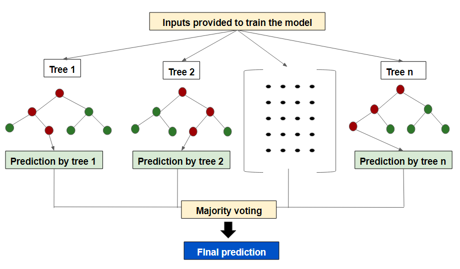
Random forest actually makes a final prediction from the prediction obtained from each of the decision tree models to overcome the weakness of a single decision tree model. In this sense, the random forest is a bagging type of ensemble technique.
We can have an idea of Random forest’s popularity by the fact that in 2010 it became the most liked machine learning in the famous data science competition website Kaggle.
The Gradient Boosting modelling was then the only other approach which came up as the closest competitor of random forest. This technique ensemble all other weak machine learning algorithms mainly decision tree. And it was quick to outperform random forest.
In Kaggle very soon gradient boosting ensemble approach overtake random forest. And still, this technique is the most used machine learning method along with the deep learning technique in almost all Kaggle competitions.
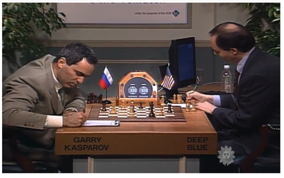
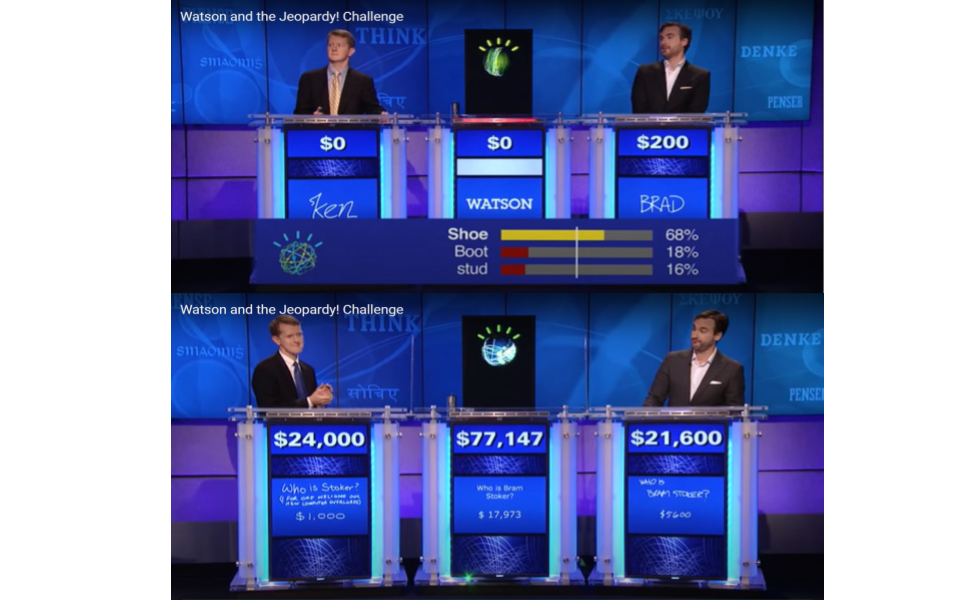
Dark Knight rises: The neural network era starts
Although the neural network was not consistent in showing its potential since 1980. Its success when demonstrated by some researchers like from IBM etc. it surprised the whole world with intelligent machines like Deep Blue, Watson etc.
The dedicated deep learning scientists putting their hard work in research never had any doubt about its potential and what it is capable of to do. The only constrain till then the research work was in very scattered form.
A coordinated research effort was very much required to establish its potential beyond any doubt. The year 2010 marked the dawn of a new era when for the first time such effort was initiated by Yann LeCun of New York University, Yoshua Bengio of the University of Montreal, Geoffrey Hinton and his group of University of Toronto and IDSIA in Switzerland.
From the group of researchers, Dan Ciresan of IDSIA first showed the world some successful applications of modern deep learning in 2011. Using his developed GPU trained deep learning network, he won some of the prestigious academic image classification competitions.
The ImageNet
ImageNet image classification competition conceptualized by Geofrey Hinton and his group from the University of Toronto started a significant chapter in the history of Deep Learning Neural Net in the year 2012.

In the same year, a team headed by Alex Krizhevsky and guided by Geoffrey Hinton recorded an accuracy of 83.6% in this image classification challenge. Which was on quite a hire side compare to the accuracy of 74.3% achieved by computer vision using classical approaches in the year 2011.
The ImageNet challenge was considered to be solved when someone with a deep convolutional network (convnets) improved the image classification accuracy up to 96.4%. Since then it was the deep convolutional neural net that had always dominated the machine learning domain.
The deep convolutional neural net got recognition by the whole world after its overwhelming success. Since then all major computer conferences and programmers meet almost all machine learning solutions are based on the deep convolutional neural net.
In some other fields like natural language processing, speech recognition also the deep convolutional neural net is a dominant technology replacing other previous tools like decision tree, SVM, random forests etc.
A good example of major players switching to deep convolutional neural net from other technologies are like the European Organization for Nuclear Research, CERN the largest particle physics laboratory in the world has ultimately switched to deep convolutional neural net to identify new particles generated from Large Hadron Collider (LHC); earlier they were using decision tree-based machine learning methods for this task.
Conclusion
The article presents a detailed history of how deep learning has made a long way to reach today’s popularity and use in many fields across different scientific disciplines. It was a journey with many peaks and valleys which started way back in 1980.
Different empirical statistical methods and machine learning algorithms preceding to deep learning made way for deep learning techniques mainly because of its high accuracy with a large amount of data.
It registered many successes and then suddenly lost in despair for not being able to meet the high expectation. It always has a true potential being more a practical technique than empirical.
Now the question is what is there in future of deep learning? What new surprises are in stock? The answer is really tough. The history we discussed here is evidence that many of them are already here to revolutionize our life.
So the next major breakthrough may also be just around the corner or it may take still years. But the field is always evolving and full of promises of blending machines with true intelligence. After all it learns from data so it will not repeat history of failures.
References
- http://www.image-net.org/
- Chollet, F., 2018. Deep Learning mit Python und Keras: Das Praxis-Handbuch vom Entwickler der Keras-Bibliothek. MITP-Verlags GmbH & Co. KG.
- https://www.wikipedia.org/
- Cortes, C. and Vapnik, V., 1995. Support-vector networks. Machine learning, 20(3), pp.273-297.
- https://www.import.io
- Vapnik, V., 1995. Support-vector networks. Machine learning, 20, pp.273-297.
- Schölkopf, B., Burges, C. and Vapnik, V., 1996, July. Incorporating invariances in support vector learning machines. In International Conference on Artificial Neural Networks (pp. 47-52). Springer, Berlin, Heidelberg.
- Rosenblatt, F., 1957. The perceptron, a perceiving and recognizing automaton Project Para. Cornell Aeronautical Laboratory.