
Multiple linear regression(MLR) is also a kind of linear regression but unlike simple linear regression here we have more than one independent variables. Multiple linear regression is also known as multivariate regression. As in real-world situation, almost all dependent variables are explained by more than variables, so, MLR is the most prevalent regression method and can be implemented through machine learning.
Mathematical equation for Multiple Linear Regression
An MLR model can be expressed as:
Yn = a0 + a1Xn1 + a2Xn2 + ⋯ + aiXi + ∈n → (Xn1 + ⋯ + Xni ) + ∈n
In the above model, the variable Yn represents response for case n and it has a deterministic part and a stochastic part; a0is the intercept, i is no. of independent variables, ai and Xi are the regression coefficients and values of independent variables, respectively and ivaries from 1 to n.
The main purpose of applying this regression technique is to develop a model which can explain the variance in the response as much as possible using the independent variables. The ratio of the explained variance by the model to the total variance of the response is known as the coefficient of determination and denoted by R2. We will discuss this statistic in detail later.
But it is an important parameter in regression modelling to ascertain how good the model is. The value of R2 varies between 0 to 1. Now three situations regarding the fitting of the model we may face which are underfitted model, good fit and overfitted model.
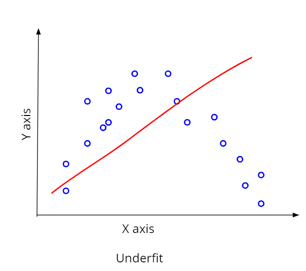
Underfit model
This situation arises when the value of R is low. Low R2 value indicates that the proposed model is not explaining the variation of the response adequately. So, the model needs improvement.
Good-fit model
Like, in this case, we have a good R2 value. Which suggests a good fit of the model and it can be used for prediction.

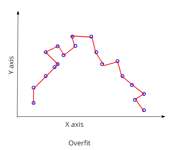
Overfit model
Sometimes models become too complex with lots of variables and parameters. Such complex models get trained by the data too well and give a very high R2 value almost close to 1.0. But they can not predict well when tested with a different set of data. This is because the model being too complex becomes too specific to a particular situation. Such models are called overfitted models.
Dataset used
The dataset used here is the same we used in the Simple Linear Regression. But in this case all the explanatory/independent variables were considered for modelling purpose. The database is an imaginary one and based on my experience of modelling tree data.
The dataset contains data on tree total biomass above the ground and several other tree physical parameters like tree commercial bole height, diameter, height, first forking height, diameter at breast height, basal area. Tree_biomass is the dependent variable here which depends on all other independent variables.
Here is a glimpse of the database:
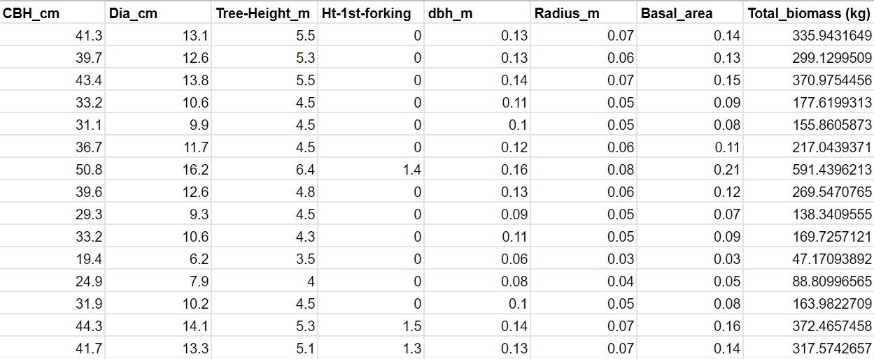
If you find any difficulty to understand the variables, just don’t bother about their names. Take them as two categories of variables, one is dependent variable, I have denoted it with y here and others are independent variable1, 2, 3 etc. Important is the relationship between these two categories of variables. Whatever their names maybe, you just have to have some experience in their relations.
Assumptions for multiple linear regression
We conduct the regression process assuming some conditions. Without holding these conditions, it is not possible to proceed with the regression process. These are called regression assumptions and they are as below:
Assumption of linearity:
There must be a linear relationship between the independent variables and the response variable. The variables in this imaginary dataset have a linear relationship between them. You can easily check this property by plotting the response variable against each of the explanatory variables.
Assumption of Homoscedasticity:
The residuals or errors that is the difference between observed and estimated values must have constant variance.
Assumption of multivariate normality:
The residuals should follow a normal distribution. We can prepare a normal quantile-quantile plot to check this assumption.
Assumption of absence of multicollinearity:
There should be no multicollinearity between the independent variables i.e. the independent variables should not be linearly related to each other.
Application of Multiple Linear Regression using Python
The main purpose of this article is to apply multiple linear regression using Python. This is the most important and also the most interesting part. So let’s jump into writing some python code. Like simple linear regression here also the required libraries have to be called first.
Calling the required libraries
We will be using fore main libraries here. For handling data frame and arrays NumPy and panda, for creating plots matplotlib and for metrics operations sklearn. These are the most important libraries for data science applications.
import numpy as np
import pandas as pd
import matplotlib.pyplot as plt
from sklearn import metrics
Importing the dataset
To import the tree dataset as mentioned earlier we will use the import function of panda library.
***** Importing the dataset ***********
dataset=pd.read_csv('tree.csv')
Defining variables
Now the next important task is to tell Python about the dependent and independent variables of the dataset. As the protocol says we will store the dependent variable in y and the independent variables in x. As I have already explained above the dataset contains one dependent variable and 7 independent variables.
So we will store the variables in two NumPy arrays. As x has to store 7 independent variables, it has to be a 2-dimensional array. Whereas being a variable with only one column, y can do with one dimension. So, the python code for this purpose is as below:
#***** Defining variables *************
x=dataset.iloc[:,: -1].values
y=dataset.iloc[:,-1].values
Here the “:” denotes the rows. As the dataset contains the dependent value i.e. tree_biomass values as the extreme right column so, python indexes it with -1.
Checking the assumption of the linear relationship between variables
For example, here I have plotted the tree_height against the dependent variable tree_biomass. Although it is evident that with the increase of tree height the biomass will certainly increase. Still, a scatterplot is a very handy visualization technique to double-check the property. You can prepare this plot very easily using the below code:
#********* Plotting dependent variable against any independent variable
plt.scatter(x[:,2],y) # accessing the variable tree_height
plt.title("Checking linearity between dependent and independent variables")
plt.xlabel("Tree height")
plt.ylabel("Tree biomass")
I have stored the variables in numpy array earlier. So, to access them we have to just mention which variable we intend to plot. For plotting we have used the plt function of matplotlib library.
And here is the plot:
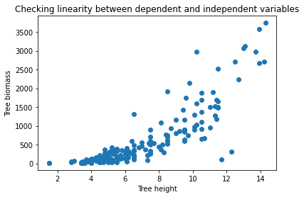
The plot suggests almost a linear relationship between the variables.
Splitting the dataset in training and test data
For testing purpose, we need to separate a part of the complete dataset which will not be used for model building. The thumb rule is to use the 80% of data for modelling and keep aside the rest of the data. It will work as an independent dataset once we come up with the model and need to test it.
#****** Dividing the dataset into training and testing dataset
from sklearn.model_selection import train_test_split
x_train, x_test, y_train, y_test= train_test_split(x, y, test_size=0.2, random_state=0)
Here this data splitting task has been performed with the help of model_selection module of sklearn library. This module has an inbuilt function called train_test_split which automatically divides the dataset into two parts. The argument test_size controls the proportion of the test data. Here it has been fixed to 0.2 so the test dataset will contain 20% of the complete data.
Application of multiple linear regression
Here comes the main part of this article that is using the regression to regress the response using the known values of more than one independent variables. As in the above section, we have already created train dataset. The following code will use this train data for model building.
#********* Application of regression
from sklearn.linear_model import LinearRegression
regressor=LinearRegression()
regressor.fit(x_train, y_train)
As it is also a linear regression method, so the linear_model module of sklearn library is the one containing the required function LinearRegression. Regressor is an instance created to apply the LinearRegression function.
Getting the regression coefficients for the regression equation
As the regression is done, we need the regression equation. This equation is actually the relation between the dependent and independent variables defined by some coefficients. Using these coefficients we can determine how a unit change in any of the independent variables is going to affect the dependent variable.
#******** Getting the coefficients stored in a dataframe
#*****************************************************************
# storing the column names of independent variables
pos=[1,2,3,4,5,6,7]
colnames=dataset.columns[pos]
print(colnames)
# creating a dataframe storing the coefficients along with the independent variable names
regressor.intercept_
coef_df=pd.DataFrame(regressor.coef_,colnames,columns=['Coefficients'])
coef_df
In the above section of code, you can see that first of all the position of the independent variables are stored in a variable. And then the corresponding coefficients are fetched from the instance regressor created from LinrarRegression function of linear_model module of sklearn. The coefficients are from regressor.coef_ and the intercept in regressor.intercept_.

The regression equation
With the help of these coefficients now we can develop the multiple linear regression.

So, this is the final equation for the multiple linear regression model.
Using the model to predict using the test dataset
Now we have the model in our hand. But how can we test its efficiency? If the model is a good one then it should have the capability to predict with precision. And to test that we will need independent data which was not involved during model building.
Here comes the role of test dataset that we kept aside at the very beginning. We will predict the response using the test dataset and compare the prediction with the observations we already have in our hand. The following code will do the trick for us.
And here is the comparison. I have created a dataframe with the observed and predicted values side by side for the ease of comparison.

In the above figure, I have shown only the first 15 values of the dataframe. But it is enough to show that the prediction is satisfactory.
Goodness of fit of the model
We have tested the data and got a good prediction using the model. However, we have not quantified yet. We do not have any number to ascertain how good is the model. Here I will discuss such fit statistics that are very useful in this respect. If we have to compare multiple models then these numbers play a crucial role to find the best out of them.
The following code will deliver fit statistics popularly used to judge the goodness of any statistical model. These are coefficient of determination denoted as R2 is the proportion of variance exists in the response variable explained by the proposed model. So the higher its value better is the model.
Coefficient of determination (R2)
Suppose our test dataset has n set of independent and dependent variables i.e. (x1,x2,…,xn), (y1,y2,…,yn)respectively. Now using our developed model the prediction we achieved has the predicted values (v1,v2,…,vn). So, the total sum of square will be:

This is the total existing variation in the response variable.
Now the variation explained by the model we developed is the regression sum of square and can be calculated as

So as the definition of the coefficient of determination goes, it can be calculated as:

Again it can be farther simplified by breaking down the regression sum of square as the variance explained subtracting the unexplained variance from the total variance. The unexplained variance is actually the variance the model is not able to explain. It is also known as error or residual sum of square and calculated as:

So, now we can rewrite the equation of R2 as

#****** Calculating fit statistics
r_square=regressor.score(x_train, y_train)
print('Coefficient of determination(R square):',r_square)
from sklearn import metrics
print('Mean Absolute Error:', metrics.mean_absolute_error(y_test, y_predict))
print('Mean Squared Error:', metrics.mean_squared_error(y_test,y_predict))
print('Root Mean Squared Error:', np.sqrt(metrics.mean_squared_error(y_test, y_predict)))
Mean Absolute Error(MAE)
This is another popular measure for model fit. As the name suggests, it is the simple difference between observed and predicted values. As we are only interested in the deviations, so we will take here the absolute value of the differences. So the expression will be:

As it measures the error of the estimated values so a lowe MAE suggests better model.
Mean Squared Error (MSE)
This is also a measure of the deviation of the model estimation from that of the original values. But instead of the absolute values, we will take the squared values of the deviations. So many a time it is also called Mean Squared Deviation (MSD) and calculated as:

Root Mean Squared Error (RMSE)
As the name suggests, this measure of fit first calculates the difference between the observed and model-predicted values, takes the square of each error then calculates the mean and ultimately calculates the square root to get the RMSE. So its equation is:


How can the fitting further be improved?
There is always scope for improving the model so that it can give more precise prediction. As we already know that the main purpose of Multiple Linear Regression is to ascribe the variance of response variable as much as possible amongst the independent variables.
Now here lies the trick of improving the prediction of multiple linear regression model. The response variable you are dealing here with gets affected by a number of explanatory variables. Some of them are straight way visible to us and we can say with confindence that they are main contributor towards the response. And all together they can give you a good explanation too.
But with a good knowledge of the domain one can identify many other variables that are not directly recognizable as causal effects. For an example if we take the example of any agriculture experiment, crop yield is determined by so many direct, indirect, physiological, chemical, weather variable, soil condition etc.
So, the skill and domain knowledge of the researcher play a viral role to choose variable wisely in order to improve the model’s fit. Using too less variable will result in a poor R2 whereas using too many variables may produce a very complex model with a very high R2. In both of these scenario model’s performance will not be up to the mark.
References:
- https://www.wikipedia.org/
- https://www.statisticshowto.com/
- https://towardsdatascience.com/